PSYC122-w19-workbook-answers

Author

Rob Davies

Introduction

In Week 19, we aim to further develop skills in working with the linear model.

We do this to learn how to answer research questions like:

What person attributes predict success in understanding?
Can people accurately evaluate whether they correctly understand written health information?

In this class, what is new is our focus on critically evaluating the ways in which people, effects or results can vary using interaction analyses.

This work simulates the kinds of interaction analyses that psychologists must often do in professional research.

Naming things

I will format dataset names like this:

all.data.csv

I will also format variable (data column) names like this: variable

I will also format value or other data object (e.g. cell value) names like this: all.data

I will format functions and library names like this: e.g. function ggplot() or e.g. library {tidyverse}.

The data we will be using

In this how-to guide, we use data from:

(1.) two 2020 studies of the response of adults from a UK national sample to written health information

study-one-general-participants.csv
study-two-general-participants.csv

(2.) along with data recently collected from PSYC122 students.

These data have been joined together to create a dataset of over 400 observations. This is because it often requires a lot of evidence to be able to draw precise or accurate conclusions about potential interaction effects.

Answers

Step 1: Set-up

To begin, we set up our environment in R.

Task 1 – Run code to empty the R environment

rm(list=ls())

Task 2 – Run code to load relevant libraries

library("ggeffects")
library("sjPlot")
library("tidyverse")

── Attaching core tidyverse packages ──────────────────────── tidyverse 2.0.0 ──
✔ dplyr     1.2.0     ✔ readr     2.1.6
✔ forcats   1.0.1     ✔ stringr   1.6.0
✔ ggplot2   4.0.2     ✔ tibble    3.3.1
✔ lubridate 1.9.4     ✔ tidyr     1.3.2
✔ purrr     1.2.1     
── Conflicts ────────────────────────────────────────── tidyverse_conflicts() ──
✖ dplyr::filter()      masks stats::filter()
✖ dplyr::lag()         masks stats::lag()
✖ ggplot2::set_theme() masks sjPlot::set_theme()
ℹ Use the conflicted package (<http://conflicted.r-lib.org/>) to force all conflicts to become errors

Step 2: Load the data

Task 3 – Read in the data file we will be using

The data file is called:

all-data.csv

Use the read_csv() function to read the data file into R:

all.data <- read_csv("all.data.csv")

Rows: 478 Columns: 11
── Column specification ────────────────────────────────────────────────────────
Delimiter: ","
chr (5): participant_ID, study, GENDER, EDUCATION, ETHNICITY
dbl (6): mean.acc, mean.self, AGE, SHIPLEY, HLVA, FACTOR3

ℹ Use `spec()` to retrieve the full column specification for this data.
ℹ Specify the column types or set `show_col_types = FALSE` to quiet this message.

Task 4 – Inspect the data file

Use the summary() function to take a look at the dataset.

summary(all.data)

 participant_ID        mean.acc        mean.self        study          
 Length:478         Min.   :0.3600   Min.   :2.250   Length:478        
 Class :character   1st Qu.:0.7500   1st Qu.:6.200   Class :character  
 Mode  :character   Median :0.8300   Median :7.200   Mode  :character  
                    Mean   :0.8066   Mean   :6.967                     
                    3rd Qu.:0.9000   3rd Qu.:7.910                     
                    Max.   :1.0000   Max.   :9.000                     
      AGE           SHIPLEY           HLVA           FACTOR3     
 Min.   :18.00   Min.   :19.00   Min.   : 2.000   Min.   : 9.00  
 1st Qu.:21.00   1st Qu.:31.00   1st Qu.: 7.000   1st Qu.:46.00  
 Median :29.00   Median :35.00   Median : 9.000   Median :50.00  
 Mean   :32.85   Mean   :34.19   Mean   : 8.929   Mean   :49.84  
 3rd Qu.:43.00   3rd Qu.:38.00   3rd Qu.:10.000   3rd Qu.:55.00  
 Max.   :76.00   Max.   :40.00   Max.   :14.000   Max.   :63.00  
    GENDER           EDUCATION          ETHNICITY        
 Length:478         Length:478         Length:478        
 Class :character   Class :character   Class :character  
 Mode  :character   Mode  :character   Mode  :character

Notice that we conducted a series of studies using the same online survey methods.

Our data include the responses made by PSYC122 students.

Step 3: Work with different kinds of variables

It is an important skill in psychological data analysis to be able to:

(1.) identify the different kinds of data variables we are working with; (2.) adapt our methods depending on differences in kind (variable Class or type).

We learn about these skills, next, in exercises that combine some revision with some new moves.

Revise: consolidate what you know

Task 5 – Use summaries or plots to examine variables

Q.1. What is the median of the FACTOR3 variable in the dataset?
A.1. You can use the summary() function to calculate that the median FACTOR3 score is 50.00
Q.2. Draw a histogram of the FACTOR3 distribution.
A.2. You can write the code as you have been shown to do previously (e.g., in week 16):

ggplot(data = all.data, aes(x = FACTOR3)) + 
  geom_histogram(binwidth = 1) +
  theme_bw() +
  labs(x = "Reading strategy (FACTOR3)", y = "frequency count")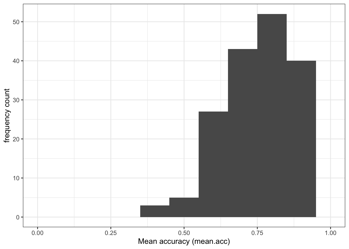

Q.3. Examine the reading strategy (FACTOR3) scores distribution: what does it tell you about the variation in the reading strategies of the participants in the sample?
A.3. The histogram shows that most participants present scores varying somewhere between 40-60 but there is a “long tail” of smaller numbers of participants with low or very low scores on the reading strategy (FACTOR3) measure.

Extend: make some new moves

We can tell from the summary and the distribution that the FACTOR3 variable consists of numbers.

Another way to identify what kind of variable we have is by using a check question:

is.factor(all.data$FACTOR3)

[1] FALSE

is.numeric(all.data$FACTOR3)

[1] TRUE

The is._() family of functions act like identity checks: what is this variable? These functions work like questions with TRUE or FALSE answers.

Is this variable a factor? [TRUE or FALSE]
Is this variable numeric? [TRUE or FALSE]

Revise: consolidate what you know

Task 6 – Identify (and change) what kind of variable – numeric or factor – a variable is

Hint: Task 6 – The `is._()` functions are available to ask what kind a variable is

Hint: Task 6 – The `as._()` functions can be used to change variable types

Q.4. What kind of variable is GENDER?
A.4. Use the same functions but change the variable name:

is.factor(all.data$GENDER)

[1] FALSE

is.numeric(all.data$GENDER)

[1] FALSE

Q.5. What do the is._() functions tell us?
A.5. The function calls tell us that GENDER is not a factor and is not numeric.
Q.6. If you look at the summary() results, what does it tell you the Class of GENDER is?
A.6. The summary shows that GENDER is identified as Class: character.

You can check this by doing the is._() test again.

is.character(all.data$GENDER)

[1] TRUE

Q.7. How do you change the class or type of the variable GENDER? Change the variable’s type (Class) into a factor.
A.7. The as._() functions can be used to change variable type, as you have done previously (e.g., in week 16).

all.data$GENDER <- as.factor(all.data$GENDER)

Q.8. What does a summary() tell us about GENDER?

summary(all.data)

 participant_ID        mean.acc        mean.self        study          
 Length:478         Min.   :0.3600   Min.   :2.250   Length:478        
 Class :character   1st Qu.:0.7500   1st Qu.:6.200   Class :character  
 Mode  :character   Median :0.8300   Median :7.200   Mode  :character  
                    Mean   :0.8066   Mean   :6.967                     
                    3rd Qu.:0.9000   3rd Qu.:7.910                     
                    Max.   :1.0000   Max.   :9.000                     
      AGE           SHIPLEY           HLVA           FACTOR3         GENDER   
 Min.   :18.00   Min.   :19.00   Min.   : 2.000   Min.   : 9.00   Female:323  
 1st Qu.:21.00   1st Qu.:31.00   1st Qu.: 7.000   1st Qu.:46.00   Male  :155  
 Median :29.00   Median :35.00   Median : 9.000   Median :50.00               
 Mean   :32.85   Mean   :34.19   Mean   : 8.929   Mean   :49.84               
 3rd Qu.:43.00   3rd Qu.:38.00   3rd Qu.:10.000   3rd Qu.:55.00               
 Max.   :76.00   Max.   :40.00   Max.   :14.000   Max.   :63.00               
  EDUCATION          ETHNICITY        
 Length:478         Length:478        
 Class :character   Class :character  
 Mode  :character   Mode  :character

A.8. The summary will show how many different participants report themselves as belonging to one of the different GENDER self-identification groups in the corresponding survey question.

You should see counts of the numbers of people in different GENDER level groups in the total survey sample:

GENDER Female:323 Male :155

We can see that 323 participants identified themselves as Female in the survey.

We can see that 155 participants identified themselves as Male in the survey.

Gender identity representation in survey samples

We note, here, that in addition to the numbers shown in the summary, six participants in the survey data entered the Non-Binary identification response option, and two participants entered the Prefer not to say option, in response to the gender identification question in the survey.

In the present exercises, we are looking at the way in which the effect on outcomes of variables – like variation in health literacy (HLVA) or reading strategy (FACTOR3) score – vary for different values of a categorical variable (like GENDER). These kinds of interactions become more complicated to analyse where there are more than two categories or levels in a factor, especially when the numbers of participants in one or more categories or levels is relatively small.

We think it is important to ensure representation of the responses and experiences of the full range of diversity among the populations we study. In future work, we hope to have collected sufficient numbers of observations from groups of participants like those entering responses like Non-Binary or Prefer not to say in order to be able to incorporate all possible between-group comparisons in analyses.

For now, we enter this explanation as a promise to to examine more representative samples in future work. Here is a link, for those who are interested, to reports of analyses of data from a survey conducted by a leading research organization (Pew Research Center). Follow the link to “Methodology” for information on how this organization exemplify good practice in obtaining representative samples.

https://www.pewresearch.org/social-trends/2025/05/29/the-experiences-of-lgbtq-americans-today/

Step 4: Now draw plots to examine associations between variables and to visualize interactions

Here, we are going to build on previous work to use plots to:

(1.) Examine the associations between pairs of variables, an outcome and a predictor (2.) Examine how the association between two variables can be different for different levels of a third variable

Scenario (2.) comes up if we are thinking about or working with interaction effects.

Consolidation: practice to strengthen skills

Task 7 – Create a scatterplot to examine the association between two numeric variables

Hint: Task 7 – We are working with `geom_point()` and you need x and y aesthetic mappings.

Here, we can look at the potential association between variation in reading strategy (using the FACTOR3 measure) and accuracy of understanding of health information (mean.acc).

Run a chunk of code to make the plot.

ggplot(data = all.data, aes(x = FACTOR3, y = mean.acc)) +
  geom_point() +
  theme_bw() +
  labs(y = "Accuracy of understanding (mean.acc)", 
       x = "Reading strategy (FACTOR3)") +
  xlim(0, 65) + ylim(0, 1)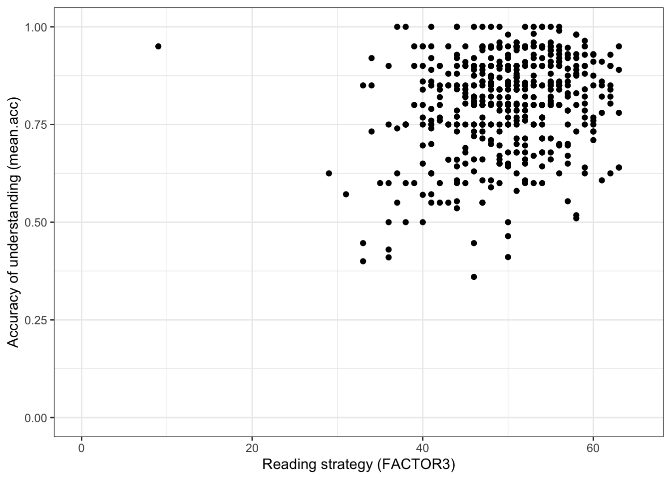

This plot shows:

the possible association between x-axis variable FACTOR3 and y-axis variable mean.acc.

The plot code moves through the following steps:

ggplot(...) make a plot;
ggplot(data = all.data, ...) with the all.data dataset;
ggplot(...aes(x = FACTOR3, y = mean.acc)) using two aesthetic mappings

x = FACTOR3 map FACTOR3 values to x-axis (horizontal, left to right) positions;
y = mean.acc map mean.acc values to y-axis (vertical, bottom to top) positions;

geom_point() show the mappings as points.
theme_bw() changes the theme to a white background.
labs(y = "Accuracy of understanding (mean.acc)", x = "Reading strategy (FACTOR3)") changes axis labels.
xlim(0, 65) + ylim(0, 1) changes axis limits.

Questions: Task 7

Q.9. What do you notice about the distribution of mean.acc scores at increasing values of reading strategy (FACTOR3) scores?
A.9. The scatterplot shows that, for increasing reading strategy (FACTOR3) scores, there is an associated rise in accuracy of understanding (mean.acc) scores.
There is extra credit for noticing that variation in outcome and predictor variable values is not tightly coupled: it is possible to have low reading strategy (FACTOR3) scores and high accuracy of understanding (mean.acc).

Introduce: make some new moves

In the next sequence of exercises, we are going to take the all.data dataset and split it into parts (sub-sets) in different ways.

We split the dataset vertically, into different sets of rows or observations.

Why are we learning how to do this?

The capacity to do this kind of split-analyse operation is extremely useful.

We are going to do this so that we can examine how the effects of interest to us (here, associations) can vary between different groups of people.

Remember, observations about different people are on different rows in all.data.
We are going to focus on an association between two column variables (mean.acc, FACTOR3).
We are going to identify different groups (sub-sets) of observations using values on a third variable.

Task 8 – Create a scatterplot to examine the association between two numeric variables, showing how the association is different for different values of a third variable

Hint: Task 8 – We are working with `geom_point()` again.

Hint: Task 8 – We can show how the association between two variables (`mean.acc`, `FACTOR3`) is different for different values of a third, categorical (factor), variable (`GENDER`) by splitting the plot so that we see the association for different levels of `GENDER`.

Here, we are splitting the dataset into:

observation data from people with just GENDER level Female
observation data from people with just GENDER level Male

and we are then producing a different scatterplot for each sub-set of data produced by the split.

Run the following chunk of code to make the plot.

ggplot(data = all.data, aes(x = FACTOR3, y = mean.acc)) +
  geom_point() +
  geom_smooth(method = 'lm') +
  theme_bw() +
  labs(y = "Accuracy of understanding (mean.acc)", 
       x = "Reading strategy (FACTOR3)") +
  xlim(0, 65) + ylim(0, 1) +
  facet_wrap(~ GENDER)

`geom_smooth()` using formula = 'y ~ x'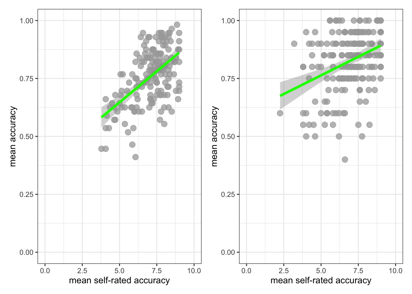

This plot shows:

the possible association between x-axis variable FACTOR3 and y-axis variable mean.acc
for different groups of people – people with self-reported GENDER responses of Female or Male.

The plot code moves through steps we have seen before. What is new here is this bit:

facet_wrap(~ GENDER)

The function facet_wrap() splits the dataset into sub-sets (different parts): different sets of rows, where different sets are defined according to different values of the variable identified inside the brackets (~ GENDER).

Here, we are asking for different scatterplots for the dataset split by whether participants are coded as Female or Male for this survey.

You can see a general guide to the function here:

https://ggplot2.tidyverse.org/reference/facet_wrap.html

Questions: Task 8

Q.10. What do you notice about the distribution of mean.acc scores at increasing values of reading strategy (FACTOR3) scores, for different sub-sets of the data: for people with Female or Male GENDER coding?
A.10. You can see that the association between mean.acc and FACTOR3 scores appears to be mostly similar for different GENDER codes.
The distribution of scores is different: we have more Female participants; their scores vary more widely.
But the trend is similar overall: the trend line representing the association between mean.acc and FACTOR3 looks similar such that for both sub-groups in the sample, increasing FACTOR3 scores are associated with higher mean.acc scores.

Hint: Task 8 – We can show how the association between two variables (`mean.acc`, `FACTOR3`) is different for different values of a third numeric variable (`HLVA`) by splitting the dataset

Here, we are first creating a new variable to code for (distinguish between) different sub-sets of observations (different rows in the dataset) based on HLVA scores, and then second drawing different plots based on different subsets.

We do this in two steps, as follows.

First, run a chunk of code to divide (cut) the dataset into parts:

all.data$HLVA_splits <- cut_number(all.data$HLVA, 3)

The code works bit-by-bit like this:

all.data$HLVA_splits <- create a new variable, HLVA_splits and add it to the dataset all.data given the work done by the bit of code on the right of the arrow <-.

On the right of the arrow <- …

cut_number(all.data$HLVA, 3) uses the cut_number(...) to divide the dataset observations into three sets based on the values in the all.data$HLVA variable named inside the brackets.

The function works by ordering all the observations (the rows) in the dataset according to the values in the named variable all.data$HLVA, then splitting the dataset (here, into three sub-sets) based on values in that named variable.

Given this code, we are going to get three sub-sets of the data, observations corresponding to (1.) low (2.) mid or (3.) high HLVA values.
We split the data into data about people with:

(1.) low HLVA values, scores between 2-8 on the HLVA test; (2.) mid HLVA values, scores between 8-10 on the HLVA test; (3.) high HLVA values, scores between 10-14 on the HLVA test.

You can see a guide to the function here:

https://ggplot2.tidyverse.org/reference/cut_interval.html

Note that where we split the data (what ranges of scores we use) will depend on the sample.

Second, we draw a plot to examine if the association between two variables (mean.acc, HLVA) is different for different values of a third variable (SHIPLEY) by splitting the data:

ggplot(data = all.data, aes(x = FACTOR3, y = mean.acc)) +
  geom_point() +
  geom_smooth(method = 'lm') +
  facet_wrap(~ HLVA_splits, nrow = 1, labeller = label_both) +
  labs(y = "Accuracy of understanding (mean.acc)", 
       x = "Reading strategy (FACTOR3)") +
  theme_bw()

`geom_smooth()` using formula = 'y ~ x'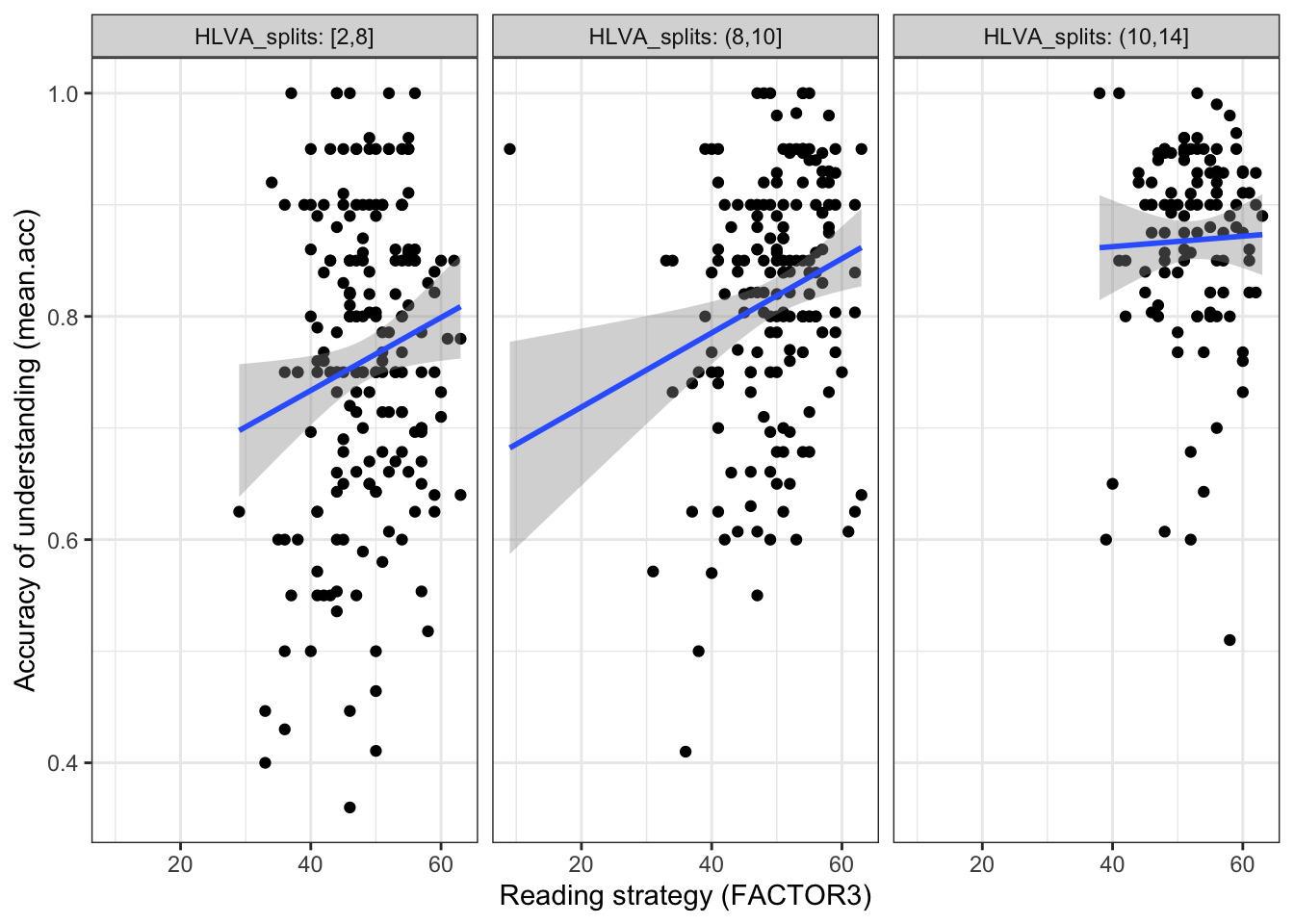

The plot code moves through the scatterplot production steps we have seen before.

The bit that is new is here:

facet_wrap(~ HLVA_splits, nrow = 1, labeller = label_both) which is included to use the data split, constructed earlier.

This addition allows us to show:

the nature of the association between two variables (mean.acc, FACTOR3)
for different values of the third variable (HLVA)
by splitting the data into three sub-sets according to HLVA score (2-8 low, 8-10 mid, 10-14 high).

Questions: Task 8

Q.11. What do you notice about the distribution of mean.acc scores at increasing values of reading strategy (FACTOR3) scores, for different sub-sets of the data: for (1.) low (2.) mid (3.) high HLVA values?
A.11. You can see that the association between mean.acc and FACTOR3 scores appears to vary (the slope differs) given different values of the third variable (HLVA).
Q.12. What do you think the values in the grey labels at the top of the facets (the plot panels) tell us?
A.12. The values tell us what values (e.g., 2,8) are used to identify the range of HLVA scores that have been used to define the sub-set of observations for which the plot below shows the association between mean.acc and FACTOR3 scores.

Step 5: Use linear models with multiple predictors, to estimate the effects of factors as well as numeric variables

Consolidation: practice to strengthen skills

As we saw in weeks 17 and 18, we can use linear models to predict outcome variables.

Linear models can include numeric variables (like FACTOR3 or HLVA) as predictors.
Linear models can also include categorical variables or factors (like GENDER or EDUCATION) as predictors.

Task 9 – First, fit a linear model including just numeric variables as predictors

Hint: Task 9 – We use the `lm()` function to fit a model with `mean.acc` as the outcome and `FACTOR3` and `HLVA` as predictors.

Note that in this model:

FACTOR3 is a measure of reading strategy – numeric scores correspond to a test of the relative effectiveness of the strategies participants use to read and understand written information;
HLVA is a measure of health literacy – numeric scores correspond to a test of knowledge of health-related words.

model <- lm(mean.acc ~ FACTOR3 + HLVA, 
            data = all.data)

summary(model)


Call:
lm(formula = mean.acc ~ FACTOR3 + HLVA, data = all.data)

Residuals:
     Min       1Q   Median       3Q      Max 
-0.38243 -0.06507  0.01136  0.07686  0.27637 

Coefficients:
             Estimate Std. Error t value Pr(>|t|)    
(Intercept) 0.4956473  0.0403305  12.290   <2e-16 ***
FACTOR3     0.0023489  0.0007874   2.983    0.003 ** 
HLVA        0.0217126  0.0024504   8.861   <2e-16 ***
---
Signif. codes:  0 '***' 0.001 '**' 0.01 '*' 0.05 '.' 0.1 ' ' 1

Residual standard error: 0.1139 on 475 degrees of freedom
Multiple R-squared:  0.1834,    Adjusted R-squared:   0.18 
F-statistic: 53.35 on 2 and 475 DF,  p-value: < 2.2e-16

If you look at the model summary you can answer the following questions.

Q.13. What is the estimate for the coefficient of the effect of the predictor, FACTOR3 (reading strategy)?
A.13. 0.0023489
Q.14. Is the effect significant?
A.14. It is significant. Because Pr(>|t|) equals 0.003 for the Estimate of the effect of FACTOR3 (reading strategy): this means that p < .05, and so the effect is significant.
Q.15. What are the values for t and p for the significance test for the estimated coefficient of the effect of HLVA (health literacy)?
A.15. t = 8.861, p = <2e-16

Hint: Task 9 – Do you know how to intepret numbers like `<2e-16`? If you are unsure you can find out about scientific notation here:

https://www.calculatorsoup.com/calculators/math/scientific-notation-converter.php

Q.16. What do you conclude are the effects of the FACTOR3 (reading strategy) and HLVA (health literacy) variables, as predictors of outcome mean.acc (accuracy of understanding of health information)?
A.16. The model slope estimates suggests that both predictors are significant, and that as both FACTOR3 (reading strategy) and HLVA (health literacy) increase, so mean.acc scores are predicted to increase also.

Task 10 – Second, fit a linear model including a numeric variable and a factor as predictors

Hint: Task 10 – We use the `lm()` function to fit a model with `mean.acc` as the outcome and `FACTOR3` and `GENDER` as predictors.

Note that in this model:

FACTOR3 is a measure of reading strategy – numeric scores correspond to a test of strategy awareness
GENDER is a self-report measure of gender identity

model <- lm(mean.acc ~ FACTOR3 + GENDER, 
            data = all.data)

summary(model)


Call:
lm(formula = mean.acc ~ FACTOR3 + GENDER, data = all.data)

Residuals:
     Min       1Q   Median       3Q      Max 
-0.43448 -0.06809  0.02190  0.09104  0.30596 

Coefficients:
              Estimate Std. Error t value Pr(>|t|)    
(Intercept)  0.6074530  0.0415532  14.619  < 2e-16 ***
FACTOR3      0.0040658  0.0008237   4.936  1.1e-06 ***
GENDERMale  -0.0108184  0.0120051  -0.901    0.368    
---
Signif. codes:  0 '***' 0.001 '**' 0.01 '*' 0.05 '.' 0.1 ' ' 1

Residual standard error: 0.1228 on 475 degrees of freedom
Multiple R-squared:  0.05007,   Adjusted R-squared:  0.04607 
F-statistic: 12.52 on 2 and 475 DF,  p-value: 5.036e-06

If you look at the model summary you can answer the following questions.

Q.17. What is the estimate for the coefficient of the effect of the predictor, FACTOR3 (strategy)?
A.17. 0.0040658
Q.18. Is the effect significant?
A.18. It is significant. Because Pr(>|t|) equals 1.1e-06 for the Estimate of the effect of FACTOR3 (strategy): this means that p < .05, and so the effect is significant.
Q.19. What are the values for t and p for the significance test for the estimated coefficient of the effect of GENDER (level, Male compared to Female)?
A.19. t = -0.901, p = 0.368
Q.20. Is the effect of GENDER significant?
A.20. It is not significant. Because Pr(>|t|) equals 0.635 for the Estimate of the effect of GENDER this means that p > .05, and so the effect is not significant.

Hint: Task 10 – How do we know how to interpret estimates for the effects of factors? We discussed how R deals with factors in week 18, and discuss factors, and the effects of factors, in the week 19 lecture.

Q.21. How should we interpret the coefficient estimate for the effect of GENDER?
A.21. Though the effect is not significant, we can say that, on average, outcome mean.acc is -0.0108184 (slightly) lower for Male compared to Female coded people.
Q.22. What do you conclude are the effects of the FACTOR3 (strategy) and GENDER (Female compared to Male) variables, as predictors of outcome mean.acc (accuracy of understanding of health information)?
A.22. The model slope estimates suggest that gender does not have a significant effect but that as FACTOR3 (strategy) scores increase, so mean.acc scores are predicted to increase.

Step 6: Use linear models with multiple predictors, including interaction effects

Introduce: make some new moves

As we saw through Task 8, it is possible that:

the association between two variables (mean.acc, FACTOR3) can be different for different values of a third categorical (factor) variable (GENDER);
the association between two variables (mean.acc, FACTOR3) can be different for different values of a third variable (HLVA)

While we can examine these possibilities using visualizations, we often need to conduct statistical analyses to test interaction effects, or the ways in which the association between two variables can be different for different levels of a third variable.

We can extend linear models to include terms that allow us to test or to estimate interaction effects.

Task 11 – Center numeric variables before using them as predictors

Hint: Task 11

When we include numeric variables (e.g., FACTOR3, HLVA, SHIPLEY) in linear models, it can cause problems of interpretation or of estimation if we include the variables as they first come to us in datasets (as raw variables).

It often helps our analyses to center variables on their means.
Centering a variable means calculating its mean, and then subtracting that mean from every value in the variable column.

For example, to center values of the HLVA variable, we create a new column data$HLVA_centered by first calculating the mean of the data$HLVA variable, and then subtracting that mean from every row value in data$HLVA.

all.data$HLVA_centered <- all.data$HLVA - mean(all.data$HLVA, na.rm = TRUE)

Q.23. Can you check what is going on when we center variables?
Hint: You can see what is happening when you run this code by first calculating the mean for HLVA

mean(all.data$HLVA, na.rm = TRUE)

[1] 8.92887

then looking at column values in the new HLVA_centered column, compared to the original HLVA column:

all.data %>%
  select(HLVA_centered, HLVA) %>%
  print(n = 20)

# A tibble: 478 × 2
   HLVA_centered  HLVA
           <dbl> <dbl>
 1       -1.93       7
 2       -0.929      8
 3        2.07      11
 4        4.07      13
 5        0.0711     9
 6       -2.93       6
 7       -1.93       7
 8       -0.929      8
 9        1.07      10
10        4.07      13
11        1.07      10
12        2.07      11
13       -0.929      8
14        1.07      10
15        1.07      10
16        1.07      10
17        3.07      12
18        1.07      10
19       -1.93       7
20       -2.93       6
# ℹ 458 more rows

What is the difference between the HLVA and HLVA_centered columns?
A.23. You can see that every value in the HLVA_centered column equals the value, on the same row, in the HLVA column, minus the mean for HLVA.
Q.24. Can you center the variable FACTOR3?
A.24. You can use the same code to center FACTOR3:

all.data$FACTOR3_centered <- all.data$FACTOR3 - mean(all.data$FACTOR3, na.rm = TRUE)

Q.25. Can you center the variable SHIPLEY?
A.25. You can use the same code to center SHIPLEY:

all.data$SHIPLEY_centered <- all.data$SHIPLEY - mean(all.data$SHIPLEY, na.rm = TRUE)

Why are we learning how to do this?

It is common in data analysis to want to transform variables before using them in analyses.

Here, we are transforming predictor variables by centering them on their mean values.

The practical reason for doing this transformation now is because if we use uncentered (raw) numeric variables as predictors in linear models that involve interactions the model can find it difficult to distinguish between the effects of those predictors and the effect of their interaction.

Task 12 – Specify models to include interaction effects: interactions between two numeric predictor variables

Hint: Task 12

We use lm() to specify models, as we have been doing.

What changes is that we now use the * operator in our model code to specify interaction effects.

For example, let’s suppose that we want to examine the possibility that the effect of reading strategy (FACTOR3) on accuracy understanding (mean.acc) is different for different values of health literacy (HLVA).

Here, we are considering the possibility that the association between reading strategy (FACTOR3) and accuracy of understanding (mean.acc) varies.
We are considering the possibility that the the association between reading strategy (FACTOR3) and accuracy of understanding (mean.acc) is different for different groups of people.
We are considering the possibility that the effect of reading strategy (FACTOR3) on accuracy of understanding (mean.acc) is different for people who differ, also, in health literacy (HLVA).

In examining the possibility that the effect of reading strategy (FACTOR3) on accuracy of understanding (mean.acc) is different for different values of health literacy (HLVA), we are examining a possible interaction between the effects of reading strategy (FACTOR3) and health literacy (HLVA).

Let’s go through this step-by-step.

First, consider: if we ignored the possibility of an interaction, we would fit a model with just the predictors: reading strategy (FACTOR3) and health literacy (HLVA).

We can fit the same model that we fit before (for Task 9).

We vary the code a little, by using the centered variables we have just created:

model <- lm(mean.acc ~ FACTOR3_centered + HLVA_centered, 
            data = all.data)

summary(model)


Call:
lm(formula = mean.acc ~ FACTOR3_centered + HLVA_centered, data = all.data)

Residuals:
     Min       1Q   Median       3Q      Max 
-0.38243 -0.06507  0.01136  0.07686  0.27637 

Coefficients:
                  Estimate Std. Error t value Pr(>|t|)    
(Intercept)      0.8065870  0.0052095 154.830   <2e-16 ***
FACTOR3_centered 0.0023489  0.0007874   2.983    0.003 ** 
HLVA_centered    0.0217126  0.0024504   8.861   <2e-16 ***
---
Signif. codes:  0 '***' 0.001 '**' 0.01 '*' 0.05 '.' 0.1 ' ' 1

Residual standard error: 0.1139 on 475 degrees of freedom
Multiple R-squared:  0.1834,    Adjusted R-squared:   0.18 
F-statistic: 53.35 on 2 and 475 DF,  p-value: < 2.2e-16

Q.26. Can you compare the summary of results for this model with the model, using the same (but not centered) predictors, that you fitted for Task 9 – compare the estimates, what do you see?
A.26. If we compare the results of the models we can see that the estimates, t-test values and probability values are the same for FACTOR3 compared to FACTOR3_centered or for HLVA compared to HLVA_centered.
This shows that centering predictors only changes the scaling of the predictor variables so that their centers are 0.

Second, now consider: we aim to test or estimate the interactions between the effects of reading strategy (FACTOR3_centered) and health literacy (HLVA_centered).

We vary the code a little, again, this time by separating the predictors by * not by +:

model <- lm(mean.acc ~ FACTOR3_centered*HLVA_centered, 
            data = all.data)

summary(model)


Call:
lm(formula = mean.acc ~ FACTOR3_centered * HLVA_centered, data = all.data)

Residuals:
     Min       1Q   Median       3Q      Max 
-0.36935 -0.06267  0.01487  0.07646  0.32573 

Coefficients:
                                 Estimate Std. Error t value Pr(>|t|)    
(Intercept)                     0.8086743  0.0053507 151.133  < 2e-16 ***
FACTOR3_centered                0.0022694  0.0007874   2.882  0.00413 ** 
HLVA_centered                   0.0213896  0.0024537   8.717  < 2e-16 ***
FACTOR3_centered:HLVA_centered -0.0005713  0.0003452  -1.655  0.09857 .  
---
Signif. codes:  0 '***' 0.001 '**' 0.01 '*' 0.05 '.' 0.1 ' ' 1

Residual standard error: 0.1137 on 474 degrees of freedom
Multiple R-squared:  0.1881,    Adjusted R-squared:  0.183 
F-statistic: 36.61 on 3 and 474 DF,  p-value: < 2.2e-16

Q.27. Can you compare the summary of results for this model with the results for the previous model (which uses the same predictors but without an interaction)?
What do you see?
A.27. If we compare the results of the models we can see that now the summary gives us estimates for the effects of:
FACTOR3_centered – this is the effect of SHIPLEY_centered when HLVA_centered is 0
HLVA_centered – this is the effect of HLVA_centered when FACTOR3_centered is 0
FACTOR3_centered*HLVA_centered – this is the interaction, and reflects the change in the effect of FACTOR3_centered on outcome mean.acc, given different values of HLVA_centered.
Notice that the effect of the interaction is not significant but that the results suggest a very slight tendencey for the effect of reading strategy to be different (smaller) for increasing values of HLVA_centered.

What are we learning here?

The * symbol (the * operator) is used here to code for a model including the effects of the two variables separated by the symbol, here, as well as the effect of the interaction between these two variables.

Task 13 – Plot model predictions to help with interpretation of interaction effects

Hint: Task 13

How do we interpret interactions?

It helps to plot model predictions, given the effects estimates that we derive from our sample using the linear model.

We can do this in a two-step sequence, similar to the sequence we trialled through weeks 17 and 18:

First fit the model
Second, use the model information to plot the predictions, given the effects

# -- first fit the model
model <- lm(mean.acc ~ FACTOR3_centered*HLVA_centered, 
            data = all.data)

# -- make plot
plot_model(model, type = "pred", 
           terms = c("FACTOR3_centered", "HLVA_centered")) +
  theme_bw() +
  ylim(0, 1)

Scale for y is already present.
Adding another scale for y, which will replace the existing scale.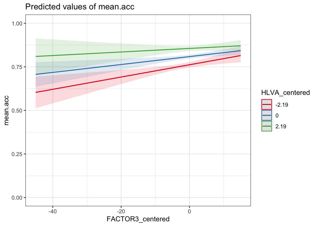

Q.28. Can you compare the summary of results for the model with the plot to develop an interpretation of the FACTOR3_centered*HLVA_centered interaction?
What do you see?
A.28. We can build an interpretation in steps:
If we look at the coefficient estimate for the FACTOR3_centered*HLVA_centered interaction, we can see that it is negative (-0.0005713).
If we look at the plot of the model predictions, we can see that there are three slopes for the FACTOR3_centered effect, one each for different levels of HLVA_centered: for HLVA_centered = -2.19; HLVA_centered = 0; and HLVA_centered = 2.19.
Notice that the steepness of the slope of the FACTOR3_centered effect decreases (the slope gets less steep) from HLVA_centered = -2.19 to HLVA_centered = 2.19.
This tells us that the interaction (though not significant) operates so that the effect of reading strategy tends to be smaller for people with higher levels of health literacy.
Returning to the fact that the coefficient estimate for the FACTOR3_centered*HLVA_centered is negative, we can now understand that it is negative because the interaction operates so that the slope of the FACTOR3_centered gets smaller as scores on HLVA_centered increase.

Task 14 – Specify models to include interaction effects: interactions between a numeric predictor variable and a factor predictor variable

Hint: Task 14 – We follow the same approach that we followed through Task 12.

Now consider: we aim to test or estimate the interactions between the effects of reading strategy (FACTOR3) and gender (GENDER).

We vary the code to change the predictor variables but the structure otherwise stays the same:

model <- lm(mean.acc ~ FACTOR3_centered*GENDER, 
            data = all.data)

summary(model)


Call:
lm(formula = mean.acc ~ FACTOR3_centered * GENDER, data = all.data)

Residuals:
     Min       1Q   Median       3Q      Max 
-0.43542 -0.07087  0.02173  0.09156  0.29573 

Coefficients:
                              Estimate Std. Error t value Pr(>|t|)    
(Intercept)                  0.8100751  0.0068412 118.412  < 2e-16 ***
FACTOR3_centered             0.0038150  0.0009700   3.933 9.64e-05 ***
GENDERMale                  -0.0109063  0.0120160  -0.908    0.365    
FACTOR3_centered:GENDERMale  0.0009027  0.0018404   0.490    0.624    
---
Signif. codes:  0 '***' 0.001 '**' 0.01 '*' 0.05 '.' 0.1 ' ' 1

Residual standard error: 0.1229 on 474 degrees of freedom
Multiple R-squared:  0.05055,   Adjusted R-squared:  0.04454 
F-statistic: 8.412 on 3 and 474 DF,  p-value: 1.86e-05

Q.29. Can you identify what effects are shown in the model summary?
A.29. We can see that now the summary gives us estimates for the effects of:
FACTOR3_centered – this is the effect of reading strategy (FACTOR3) when GENDER level is Female
GENDERMale – this is the effect of GENDER when FACTOR3_centered is 0.

Note that the effect of GENDER is the estimated difference in outcome when GENDER level is Female (not shown, treated as the baseline) compared to when GENDER level is Male.

FACTOR3_centered*GENDER – this is the interaction, and reflects the change in the effect of FACTOR3_centered on outcome mean.acc, given different values of GENDER, here, when GENDER is Male instead of Female.

What are we learning here?

Remember from week 18:

Categorical variables or factors and reference levels.

If you have a categorical variable like GENDER then when you use it in an analysis, R will look at the different categories (called levels) e.g., here,Female, Male` and it will pick one level to be the reference or baseline level.
The reference is the the level against which other levels are compared.
Here, the reference level is Female simply because, unless you tell R otherwise, it picks the level with a category name that begins earlier in the alphabet as the reference level.

How do we interpret interactions?

It helps to plot the effects estimates, given the model.

We can do this in a two-step sequence, similar to the sequence we trialled through weeks 17 and 18:

First fit the model
Second, use the model information to plot the predictions, given the effects

# -- first fit the model
model <- lm(mean.acc ~ FACTOR3_centered*GENDER, 
            data = all.data)

# -- make plot
plot_model(model, type = "pred", 
           terms = c("FACTOR3_centered", "GENDER")) +
  theme_bw() +
  ylim(0, 1)

Scale for y is already present.
Adding another scale for y, which will replace the existing scale.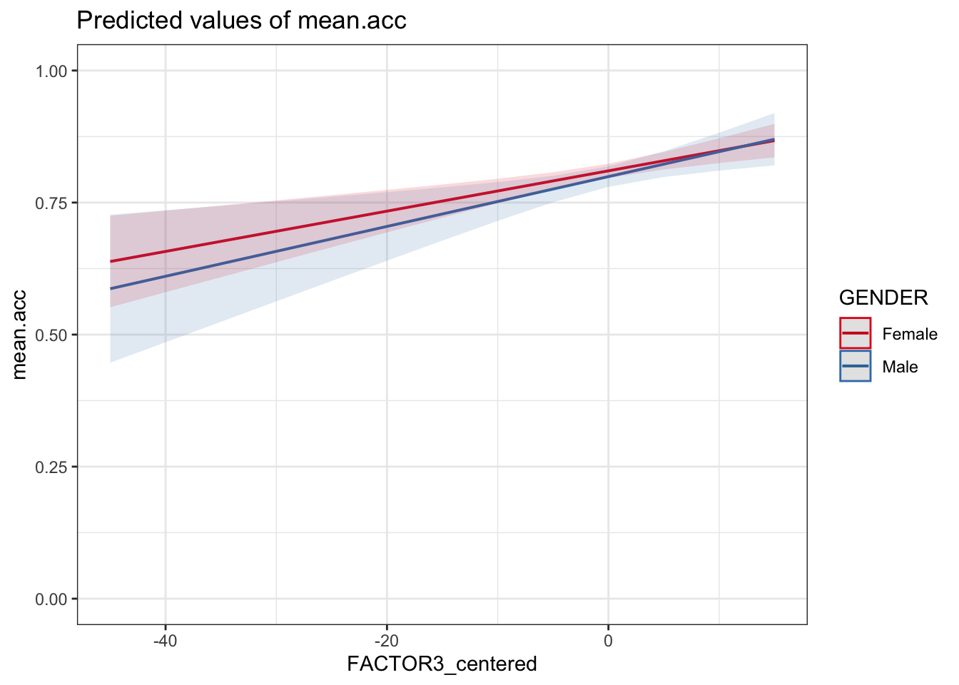

Q.30. Can you identify how the effects of reading strategy (FACTOR3) and gender (GENDER) interact, given the model results summary and this plot?
A.30. The plot, and the estimate for the interaction FACTOR3_centered:GENDERMale, together show that the coefficient for the effect of reading strategy (FACTOR3_centered) is slightly larger (the slope is slightly steeper) when GENDER is Male instead of `Female.
Notice that, for this sample, the interaction is not significant, suggesting that there is no difference between genders in the relative effectiveness of reading strategy.

Introduction

Naming things

The data we will be using

Answers

Step 1: Set-up

Task 1 – Run code to empty the R environment

Task 2 – Run code to load relevant libraries

Step 2: Load the data

Task 3 – Read in the data file we will be using

Task 4 – Inspect the data file

Step 3: Work with different kinds of variables

Revise: consolidate what you know

Task 5 – Use summaries or plots to examine variables

Extend: make some new moves

Revise: consolidate what you know

Task 6 – Identify (and change) what kind of variable – numeric or factor – a variable is

Hint: Task 6 – The is._() functions are available to ask what kind a variable is

Hint: Task 6 – The as._() functions can be used to change variable types

Gender identity representation in survey samples

Step 4: Now draw plots to examine associations between variables and to visualize interactions

Consolidation: practice to strengthen skills

Task 7 – Create a scatterplot to examine the association between two numeric variables

Hint: Task 7 – We are working with geom_point() and you need x and y aesthetic mappings.

Questions: Task 7

Introduce: make some new moves

Why are we learning how to do this?

Task 8 – Create a scatterplot to examine the association between two numeric variables, showing how the association is different for different values of a third variable

Hint: Task 8 – We are working with geom_point() again.

Hint: Task 8 – We can show how the association between two variables (mean.acc, FACTOR3) is different for different values of a third, categorical (factor), variable (GENDER) by splitting the plot so that we see the association for different levels of GENDER.

Questions: Task 8

Hint: Task 8 – We can show how the association between two variables (mean.acc, FACTOR3) is different for different values of a third numeric variable (HLVA) by splitting the dataset

Questions: Task 8

Step 5: Use linear models with multiple predictors, to estimate the effects of factors as well as numeric variables

Consolidation: practice to strengthen skills

Task 9 – First, fit a linear model including just numeric variables as predictors

Hint: Task 9 – We use the lm() function to fit a model with mean.acc as the outcome and FACTOR3 and HLVA as predictors.

Hint: Task 9 – Do you know how to intepret numbers like <2e-16? If you are unsure you can find out about scientific notation here:

Task 10 – Second, fit a linear model including a numeric variable and a factor as predictors

Hint: Task 10 – We use the lm() function to fit a model with mean.acc as the outcome and FACTOR3 and GENDER as predictors.

Hint: Task 10 – How do we know how to interpret estimates for the effects of factors? We discussed how R deals with factors in week 18, and discuss factors, and the effects of factors, in the week 19 lecture.

Step 6: Use linear models with multiple predictors, including interaction effects

Introduce: make some new moves

Task 11 – Center numeric variables before using them as predictors

Hint: Task 11

Why are we learning how to do this?

Task 12 – Specify models to include interaction effects: interactions between two numeric predictor variables

Hint: Task 12

What are we learning here?

Task 13 – Plot model predictions to help with interpretation of interaction effects

Hint: Task 13

Task 14 – Specify models to include interaction effects: interactions between a numeric predictor variable and a factor predictor variable

Hint: Task 14 – We follow the same approach that we followed through Task 12.

What are we learning here?

How do we interpret interactions?

Hint: Task 6 – The `is._()` functions are available to ask what kind a variable is

Hint: Task 6 – The `as._()` functions can be used to change variable types

Hint: Task 7 – We are working with `geom_point()` and you need x and y aesthetic mappings.

Hint: Task 8 – We are working with `geom_point()` again.

Hint: Task 8 – We can show how the association between two variables (`mean.acc`, `FACTOR3`) is different for different values of a third, categorical (factor), variable (`GENDER`) by splitting the plot so that we see the association for different levels of `GENDER`.

Hint: Task 8 – We can show how the association between two variables (`mean.acc`, `FACTOR3`) is different for different values of a third numeric variable (`HLVA`) by splitting the dataset

Hint: Task 9 – We use the `lm()` function to fit a model with `mean.acc` as the outcome and `FACTOR3` and `HLVA` as predictors.

Hint: Task 9 – Do you know how to intepret numbers like `<2e-16`? If you are unsure you can find out about scientific notation here:

Hint: Task 10 – We use the `lm()` function to fit a model with `mean.acc` as the outcome and `FACTOR3` and `GENDER` as predictors.