122_wk13_labActivity2

Author

Margriet Groen

Published

January 24, 2024

Lab activity 2 - Reminders through association

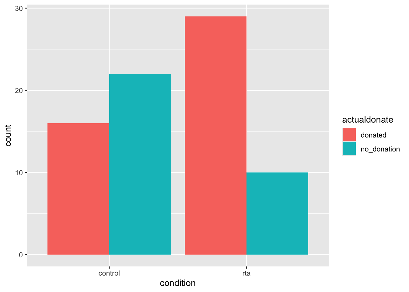
Aim: What we want to do is to run a chi-square analysis to determine whether those in the RTA condition were more likely to remember to return the paper-clips than those in the control condition.

Step 1. Loading the relevant libraries

library(lsr)
library(tidyverse)

── Attaching core tidyverse packages ──────────────────────── tidyverse 2.0.0 ──
✔ dplyr     1.2.0     ✔ readr     2.1.6
✔ forcats   1.0.1     ✔ stringr   1.6.0
✔ ggplot2   4.0.2     ✔ tibble    3.3.1
✔ lubridate 1.9.4     ✔ tidyr     1.3.2
✔ purrr     1.2.1     
── Conflicts ────────────────────────────────────────── tidyverse_conflicts() ──
✖ dplyr::filter() masks stats::filter()
✖ dplyr::lag()    masks stats::lag()
ℹ Use the conflicted package (<http://conflicted.r-lib.org/>) to force all conflicts to become errors

Step 2. Read in the data and have a look at it

intent_data <- read_csv("RTA_study1.csv")                                 # Read in the data file

Rows: 87 Columns: 4
── Column specification ────────────────────────────────────────────────────────
Delimiter: ","
dbl (4): condition, intend, actualdonate, id

ℹ Use `spec()` to retrieve the full column specification for this data.
ℹ Specify the column types or set `show_col_types = FALSE` to quiet this message.

head(intent_data)                                                         # Look at the table

# A tibble: 6 × 4
  condition intend actualdonate    id
      <dbl>  <dbl>        <dbl> <dbl>
1         1      1            1     1
2         1      1            1     2
3         1      1            1     3
4         1      1            1     4
5         1      1            1     5
6         1      1            1     6

Question 2a: What do the numbers in the first row across the four columns refer to?

condition = 1, intend = 1, actualdonate = 1 and id = 1 shows us that participant 1 was in the ‘reminder-through-assocation’ condition, reported that they intended to donate and also actually donated.

Step 3. Getting the data ready.

intent_recode <- intent_data %>%
  filter(intend == 1) %>%
  mutate(condition = recode(condition, "1" = "rta", "2" = "control"),
         actualdonate = recode(actualdonate, "1" = "donated", "0" = "no_donation"))

head(intent_recode)

# A tibble: 6 × 4
  condition intend actualdonate    id
  <chr>      <dbl> <chr>        <dbl>
1 rta            1 donated          1
2 rta            1 donated          2
3 rta            1 donated          3
4 rta            1 donated          4
5 rta            1 donated          5
6 rta            1 donated          6

Question 3a: How many participants were removed because they didn’t intend to return the paper-clips? 10 participants. The table ‘intent_data’ contains 87 observations, after we have applied the filter() function to include only those participants who did intend to return the paper-clips, the intent_recode table contains 77 observations.

Step 4: Calculating descriptive statistics

intent_counts <- intent_recode %>%
group_by(condition, actualdonate) %>%
  count()

intent_counts

# A tibble: 4 × 3
# Groups:   condition, actualdonate [4]
  condition actualdonate     n
  <chr>     <chr>        <int>
1 control   donated         16
2 control   no_donation     22
3 rta       donated         29
4 rta       no_donation     10

Question 4a: How many participants in the control condition didn’t donate? 22

Question 4b: How many participants in the control condition donated? 16

Question 4c: How many participants in the rta condition didn’t donate? 10

Question 4d: How many participants in the rta condition donated? 29

Percentages

intent_percent <- intent_recode %>%
  group_by(condition, actualdonate) %>%
  count() %>%
  ungroup() %>% # ungroups the data
  group_by(condition) %>% # then groups it again but just by condition
  mutate(percent_condition = n/sum(n) * 100)

intent_percent

# A tibble: 4 × 4
# Groups:   condition [2]
  condition actualdonate     n percent_condition
  <chr>     <chr>        <int>             <dbl>
1 control   donated         16              42.1
2 control   no_donation     22              57.9
3 rta       donated         29              74.4
4 rta       no_donation     10              25.6

Step 5: Visualise the data

ggplot(data = intent_recode, aes(x = condition, fill = actualdonate)) +
  geom_bar(position = "dodge")

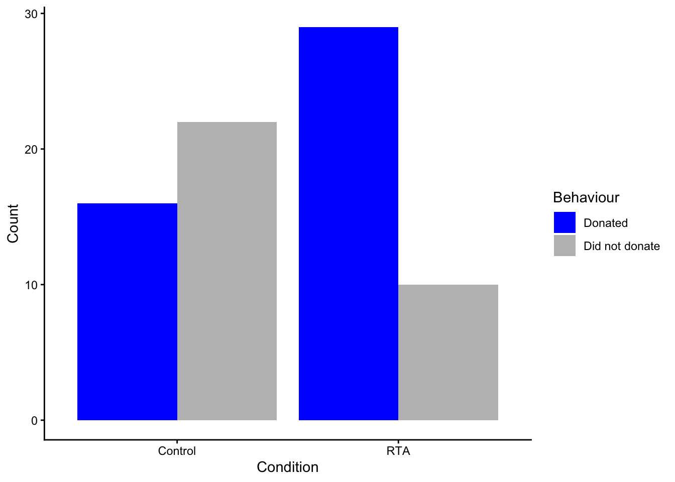
Question 5a: What does position = "dodge" do? Remove it and rerun the code to find out. “dodge” places the bars next to each other, rather than on top of each other.

ggplot(data = intent_recode, aes(x = condition, fill = actualdonate)) + # sets up the base of the graph: the data to use and the aesthetics (what will go on the x
# and y axis, how the plot will be grouped
  geom_bar(position = "dodge") + # places the bars next to each other, rather than on top of each other.
  scale_x_discrete(name = "Condition", labels = c("Control", "RTA")) + # relabels categories on x axis
  scale_y_continuous(name = "Count") + # relabels y axis
  scale_fill_manual(name = "Behaviour", labels = c("Donated", "Did not donate"), values = c("blue", "grey"))+ # labels colour legend labels and uses colours blue and grey
  theme_classic() #changes the background

Step 6: Run Chi-square test ———————————-

results <- chisq.test(x = intent_recode$condition,        # the first grouping variable
                      y = intent_recode$actualdonate,     # the second grouping variable
                      correct = FALSE)                    # whether we want to apply the continuity correction (use if any of the expected cell frequencies < 10 in 2 x 2 table)
results


    Pearson's Chi-squared test

data:  intent_recode$condition and intent_recode$actualdonate
X-squared = 8.244, df = 1, p-value = 0.004089

Question 6a: What do you conclude from the output? There is a significant association between the grouping variables.

Step 7: Checking assumptions

The assumptions for chi-square are as follows:

The data in the cells should be frequencies, or counts of cases rather than percentages. As long as you have used the correct data frame this assumption is satisfied.
The levels (or categories) of the variables are mutually exclusive. That is, a particular participant fits into one and only one group of each of the variables. This is true for this experiment.
Each participant may contribute data to one and only one cell. If, for example, the same participants are tested over time such that the comparisons are of the same subjects at Time 1, Time 2, Time 3, etc., then Chi-square may not be used. This is true for this experiment.
The study groups must be independent. This means that a different test must be used if the two groups are related. For example, a different test must be used if the researcher’s data consists of paired samples, such as in studies in which a parent is paired with his or her child. The groups in this experiment are independent.
There are 2 variables, and both are measured as categories, usually at the nominal level. While Chi-square has no rule about limiting the number of cells (by limiting the number of categories for each variable), a very large number of cells (over 20) can make it difficult to meet assumption #6 below, and to interpret the meaning of the results. This is true for this experiment.
The expected cell frequencies should be greater than 5.

Assumptions 1) to 5) should be evaluated by reviewing the design of the study. The only assumption that we need to check with R is whether all expected frequencies are greater than 5.

results$expected

                       intent_recode$actualdonate
intent_recode$condition  donated no_donation
                control 22.20779    15.79221
                rta     22.79221    16.20779

Question 7a: What do you conclude from the output? The expected frequencies in all cells are greater than 5.

Step 8: Effect size

Cramer’s V

eff_size <- cramersV(x = intent_recode$condition,     # the first grouping variable
                     y = intent_recode$actualdonate  # the second grouping variable
                     )                  # whether we want to apply the continuity correction (use if any of the expected cell frequencies < 10 in 2 x 2 table)
eff_size

[1] 0.327207

Percentage variance accounted for:

percentageAccountedFor <- eff_size * eff_size * 100
percentageAccountedFor

[1] 10.70644

Question 8a: How large is the effect and how much variance is accounted for? The effect size (Cramer’s V) = 0.33 and the percentage variance accounted for = 11%.

Step 9: Standardised residuals

results$residuals   # check the standardised residuals

                       intent_recode$actualdonate
intent_recode$condition   donated no_donation
                control -1.317299    1.562125
                rta      1.300301   -1.541968

Question 9a: What do you conclude from the output? The standardised residuals in the 4 cells are all of a roughly similar size (and below 1.96), which suggests that the statistically significant Chi-square tests is not driven by one or two cells, but reflects the pattern across all cells.

Step 10: Write up

Those in the reminder-through-association condition performed the intended behaviour at a significantly higher rate (74%, 29 out of 39) than did those in the control condition (42%, 16 out of 38)), χ2(1, N = 77) = 8.24, p = 0.004, V = 0.33. The analysis showed that 11% of variance in intended behaviour could be accounted for by condition (reminder-through-association vs. control).