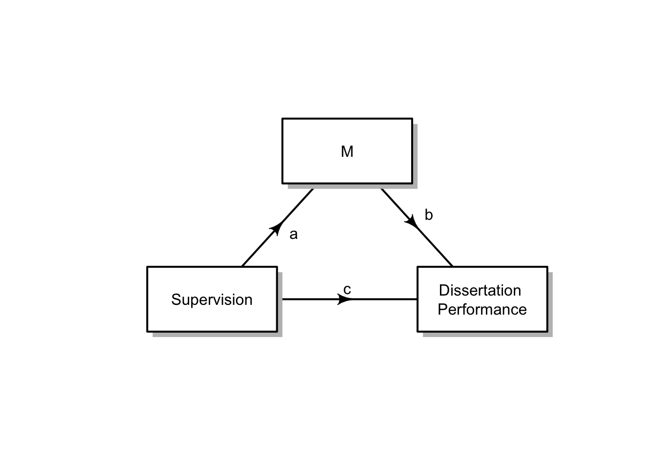
Early in the construction of the script, I noticed that there were different levels of missingness across the models - this means that coefficients are estimated on different datasets, so we are introducing a potential source of systematic error if we do not correct for this.
Checking for missingness:
summary(d_full)
  supervision     self_esteem    dissertation_performance
 Min.   :1.667   Min.   :1.571   Min.   :1.000
 1st Qu.:3.333   1st Qu.:3.286   1st Qu.:2.380
 Median :4.000   Median :3.857   Median :3.037
 Mean   :3.786   Mean   :3.864   Mean   :3.028
 3rd Qu.:4.333   3rd Qu.:4.500   3rd Qu.:3.593
 Max.   :5.000   Max.   :5.714   Max.   :5.815
                 NA's   :2       NA's   :3
For the purposes of this analysis, I will remove the observations (rows) with NA values. This is not the best way of working with missingness, but for the purposes of the demonstration it is ok.
d <-na.omit(d_full) # 4 observations removedsummary(d) # no NA values listed
  supervision     self_esteem    dissertation_performance
 Min.   :1.667   Min.   :1.571   Min.   :1.000
 1st Qu.:3.333   1st Qu.:3.286   1st Qu.:2.370
 Median :4.000   Median :3.857   Median :3.074
 Mean   :3.791   Mean   :3.853   Mean   :3.030
 3rd Qu.:4.333   3rd Qu.:4.429   3rd Qu.:3.593
 Max.   :5.000   Max.   :5.714   Max.   :5.815
I am going to copy and rename the variables to save on typing
X = supervision Y = dissertation_performance M = self_esteem
d <- d %>%mutate(X = supervision,Y = dissertation_performance,M = self_esteem)
Longhand - Steps of Baron & Kenny (1986)
Four independent linear regression models
The effect of X on Y (total effect = pathway c)
The effect of X on M (indirect effect pathway a)
The effect of M on Y (indirect effect pathway b) while controlling for X
The effect of X and M on Y (for direct effect estimation = pathway c’)
When running your models, you need to assign them to objects in the environment to then be able to use them in a call to the mediation package.
Step 1: Test the total effect - pathway c
\[
Y = b_0 + b_1 * X + e
\]
via a simple regression model:
(fit_total <-summary(lm(Y ~ X, d)))
Call:
lm(formula = Y ~ X, data = d)

Residuals:
     Min       1Q   Median       3Q      Max
-1.83011 -0.56623 -0.04308  0.51478  2.25553

Coefficients:
            Estimate Std. Error t value Pr(>|t|)
(Intercept)   1.3718     0.4679   2.931 0.004470 **
X             0.4375     0.1209   3.620 0.000532 ***
---
Signif. codes:  0 '***' 0.001 '**' 0.01 '*' 0.05 '.' 0.1 ' ' 1

Residual standard error: 0.8361 on 75 degrees of freedom
Multiple R-squared:  0.1488,    Adjusted R-squared:  0.1374
F-statistic: 13.11 on 1 and 75 DF,  p-value: 0.0005321
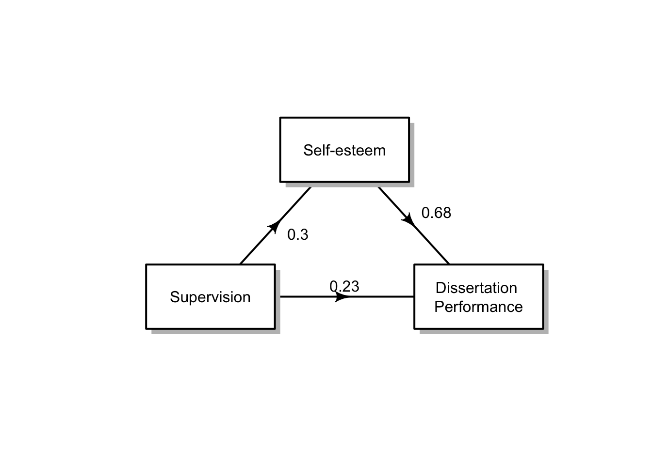
The total effect of our predictor on our outcome is significant. In other words, supervision on dissertation performance is significant (p < .001). A change in one unit of supervision is associated with an increase in dissertation performance of 0.44.
There is an effect that can be tested for mediation.
Step 2: Test the a pathway of the indirect effect
\[
M = b_0 + b_1 * X + e
\] a second simple regression model, using X as a predictor but this time, M (self esteem here) is our outcome variable:
(fit_indirecta <-summary(lm(M ~ X, d)))
Call:
lm(formula = M ~ X, data = d)

Residuals:
     Min       1Q   Median       3Q      Max
-2.34553 -0.48838  0.02337  0.61288  1.49353

Coefficients:
            Estimate Std. Error t value Pr(>|t|)
(Intercept)   2.7018     0.4406   6.132 3.74e-08 ***
X             0.3038     0.1138   2.670   0.0093 **
---
Signif. codes:  0 '***' 0.001 '**' 0.01 '*' 0.05 '.' 0.1 ' ' 1

Residual standard error: 0.7872 on 75 degrees of freedom
Multiple R-squared:  0.08679,   Adjusted R-squared:  0.07461
F-statistic: 7.128 on 1 and 75 DF,  p-value: 0.0093
The indirect effect pathway a (X on M) is also significant (p = .009). A change in one unit of supervision is associated with an increase in self-esteem of 0.30.
So now we know that X and M share some variance - they are correlated. We have met one of the assumptions that we need to be able to perform a mediation analysis.
Step 3 & 4: Test the b pathway of the indirect effect & the direct effect (pathway c’)
\[
Y = b_0 + b_1 * X + b_2 * M + e
\] A multiple regression model, with Y (dissertation performance) as our outcome variable, and X (supervision) and M (self-esteem) as predictors. Remember that this model is controlling for the effect of X on Y, because interpreting one predictor in a multiple regression model always assumes that the effect of the other predictors are already taken care of, or controlled for.
(fit_indirectb <-summary(lm(Y ~ X + M, d)))
Call:
lm(formula = Y ~ X + M, data = d)

Residuals:
     Min       1Q   Median       3Q      Max
-1.39749 -0.48798  0.02245  0.44603  1.29565

Coefficients:
            Estimate Std. Error t value Pr(>|t|)
(Intercept) -0.46168    0.44402  -1.040   0.3018
X            0.23135    0.09794   2.362   0.0208 *
M            0.67861    0.09497   7.145 5.26e-10 ***
---
Signif. codes:  0 '***' 0.001 '**' 0.01 '*' 0.05 '.' 0.1 ' ' 1

Residual standard error: 0.6475 on 74 degrees of freedom
Multiple R-squared:  0.4963,    Adjusted R-squared:  0.4827
F-statistic: 36.46 on 2 and 74 DF,  p-value: 9.564e-12
The indirect effect pathway b (M on Y), while controlling for X is also significant (p < .001). A change in one unit of self-esteem is associated with an increase in dissertation-performance of 0.68 of a unit. The predictor (X) relationship with the outcome (Y and pathway c’ - the direct effect) remains significant also (p < .02 , but reduced relative to the step 1 model coefficient (step 1 \(b\) = 0.44, step 4 \(b\) = 0.23).
Since the direct pathway c’ is significant, we can say that we have a partially mediated effect of self-esteem on the relationship between supervision and dissertation performance. Supervision predicts self esteem and dissertation performance, while self esteem also predicts dissertation performance.
If instead the X coefficient in the model above had been > .05 i.e. no significant, we could have claimed a full or complete mediation of self esteem on the relationship between supervision and dissertation performance
Using the power of R and the mediation package
The mediation package is called by the library() function loaded at the top of the document.
It takes the models for pathways a and b (fit_indirecta and fitindirectb here),
It needs us to tell it the name of the predictor or treatment variable and the name of the mediator variable as labelled in the models
and we set the boot argument to T for TRUE, to be able to generate confidence intervals on our co-efficients.
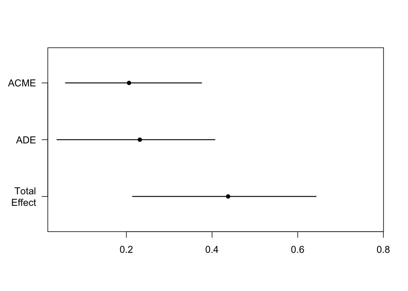
ACME stands for average causal mediation effects and is the product of pathway a and pathway b from fit indirecta (X = 0.3037992) and fit_indirectb (M = 0.6786069).
ADE stands for average direct effects or pathway c’. This is the X coefficient in our fit_indirectb
Total Effect does what it says on the tin. It is the sum of the direct and indirect effect, ACME + ADE, and also calculated as X in model fit_total.
Prop. Mediated is the proportion of the effect of X on Y that goes through M. We divide ACME (or ab) by the total effect (c).
plot(results)
Reporting the mediation analysis
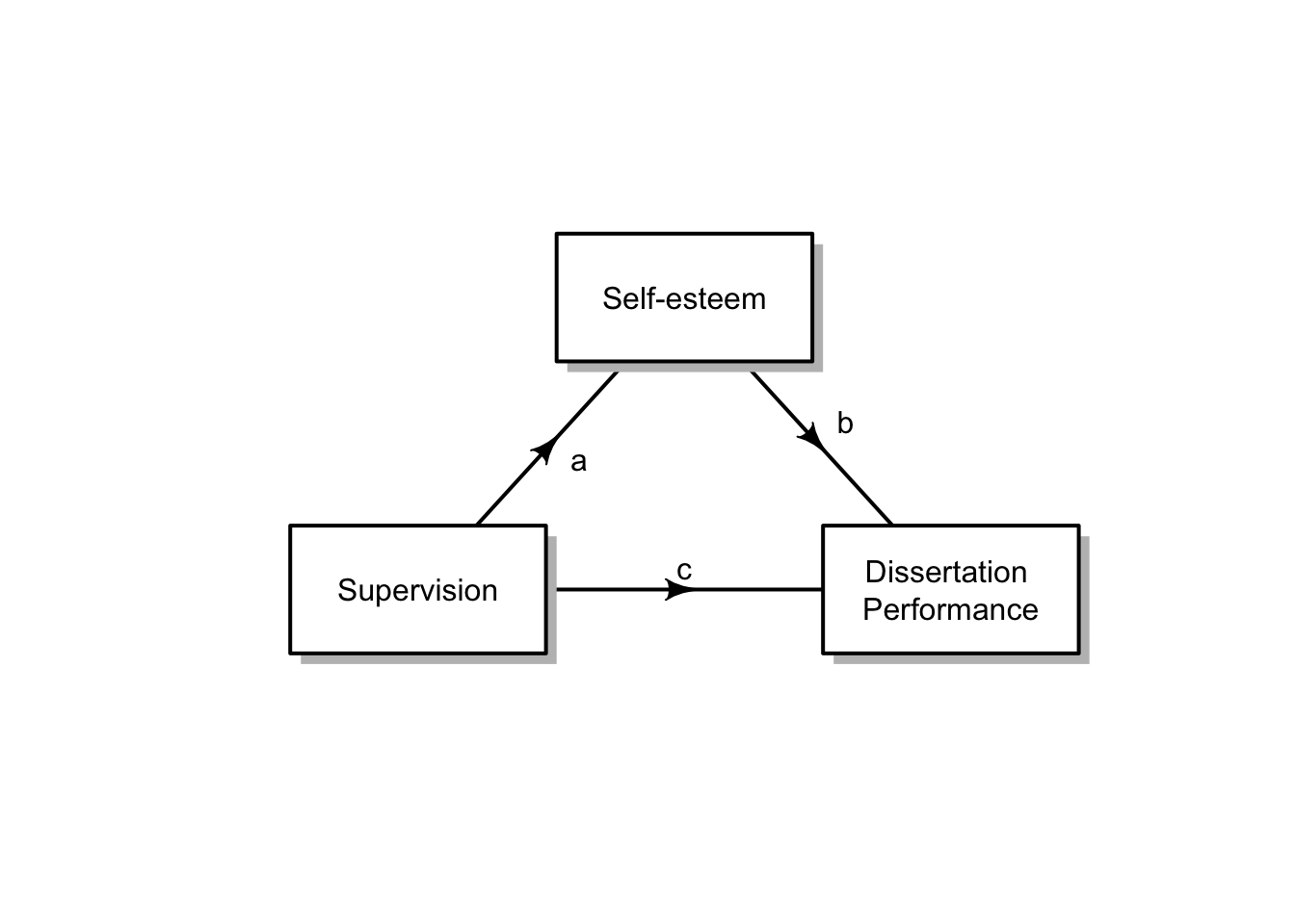
and to use our diagram from the top of the document:
We are going to test for the mediator variable of self esteem. (This needs the prime mark added to the direct pathway “c” text!)
(Remember that these data are not standardised so we cannot compare between them for strength of relationships!)
The effect of supervision on dissertation performance was partially mediated via self-esteem. The effect of supervision on dissertation performance and the effect of self-esteem on dissertation performance were independently significant predictors. The indirect effect equals (.3)*(0.68) = .0.21. We tested the significance of this indirect effect using bootstrapping procedures. We computed the average indirect effect over 1,000 bootstrapped samples with 95% confidence intervals (bootstrapped indirect effect = 0.21 95% CI [0.06, 0.38]). Since the confidence intervals do not cross zero, we infer statistical significance.