1. Review of correlation, simple regression and demonstration of multiple regression
Emma Mills
Lecture
The lecture for week 11 is here. Please note, it is best to view the video using the screen viewer. That way you see the moving cursor and when I move to the RStudio demonstration at around 37 minutes, you will see everything. If you have the slide viewer selected, then around 37 minutes, you will need to move to the screen view so that you can see the RStudio demonstration.
Materials
There are two folders to download for week 11: I separated the materials into files that R will upload, or should upload with no error; and .docx or .pdf files that R would not like. Please store the second folder somewhere for your use.
- The first folder is a zipped folder called Week 11 234 Materials.zip. It can be downloaded here. You can upload the zip file directly on to the R server and it will populate a new folder with the files and data files automatically.
- The second folder is called “Week_11_234_Slides_Codebook.zip”. The slides are for the lecture; the Codebook is paired with the “student-por.csv” dataset. We will be looking at a model output for this dataset in the lab. Please download here.
Pre-Lab Activity
Please download the Week 11 materials (link above) and upload all of the .Rmd files and data files to your R account in preparation for the lab.
Please run through the three .Rmd files listed below by yourself. These all depend on the Covariance.csv data file
- Correlation Review
- Simple Regression Review
- Multiple Regression Review
- Look at the “Planning ANY Data Analysis” slides which are related to the lab in Week 11.
Recommended Reading
Chapters 9, 10 and 11 from Howell, D. C. (2017). Fundamental statistics for the behavioral sciences (Ninth edition.). Cengage. There are online versions available from the library at this link
Test Yourself!
The link to this week’s multiple choice quiz is here
Overview of Learning Model in 234
What happens?
Before the lab
watch the weekly lecture
- Seriously, there is no point coming to the lab if you haven’t watched the lecture.
In each lab
- You will be given a dataset and model summary
- Each week’s model summary will include practice of the new parts of learning featured in the week’s lecture
- In small groups, write the script that produced the model output
- You can connect one computer to the big screen at the table in the Levy lab, and work together by looking at that script while finding code that works on personal laptops.
- Use the analysis workflow diagram and process (see below)
- Talk together about the model summary first
- Interpret it so you have a working understanding of what you are going to be preparing
- Look at which variables have been used in the model
- If there is a codebook, use the codebook to understand what each variable represents
- Create some possible hypotheses that the model seeks to explain
- Collaborate in writing the script
- You can scrape code from all your statistics modules and the web
- The internet
- R books
- You can scrape code from all your statistics modules and the web
- Refer to the demonstration script from the lecture
- Use the lab time and staff to check your plan / process
- Independent study time:
- Continue to work on the script if you want to foster that independence.
- Submit for feedback
- If you want some feedback on what you consider a completed script, please send forward to e.mills@lancaster.ac.uk or alternatively, you could post snippets of code for which you want feedback on the moodle discussion forum. These don’t have to be perfect! Coding is a process and can always be improved, consequenty it’s always imperfect and unfinished. I encourage you to be brave.
- remember to attach your R script if you are emailing!
- Model scripts
- At the end of each lab, we will run through together a set of possible ways of approaching an analysis that gives us the model summary output
- A model script showing one way of answering the research questions will be published in the following week on the respective lecture pages.
Data Analysis
Any good data analysis requires the following steps:
Importing the data
Tidying or cleaning the data
Performing any necessary transformations
Visualising the data
Modelling the data
Communicating the findings from the data
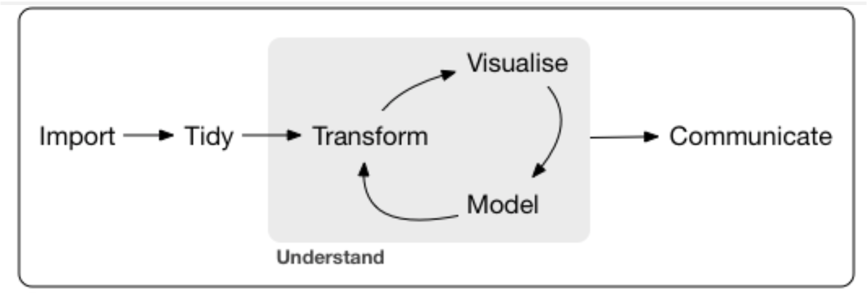
These steps may be familiar to you and are represented in the diagram below:

You may remember the diagram itself from PSYC 122 and PSYC 214. Each step of the plan requires its own mini block of code that you will need to include in your scripts.
Also, multiple regression, the focus model of PSYC 234, uses data that has many variables - hence the label ‘multiple’ - and the analysis that we may need to complete may be quite complex.
Because the data has many variables, using raw data may mean that the first model we execute makes no sense and is hard to interpret. If a model is hard to interpret is it going to be even harder to communicate to a naive audience. For this reason, we will learn about some very useful transformations over the next few weeks. For one analysis, we may go around the Visualise-Transform-Model part of the diagram more than once before we have a model that we can interpret and communicate.
Critically, performing these transformations does not change the information that is in the data and the relationships that exist between all the variables in the raw data. The change that we see through using these transformations is only in the final expression of the model. The transformations will assist in making a model that makes more sense with what we observe in everyday life. I will point this out as we see examples of this over the next few weeks.
Reporting a Linear Regression Analysis

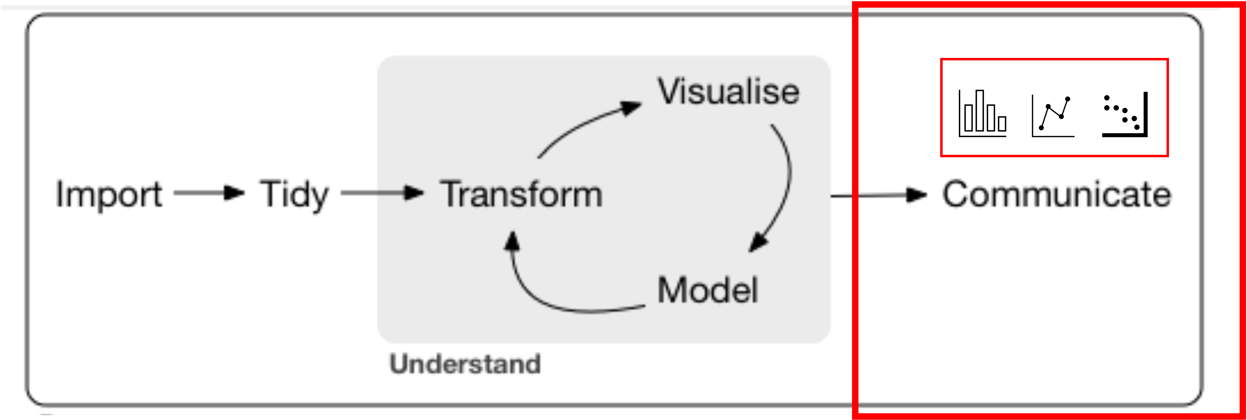
Additionally, the communication step of the workflow requires us to visualise the findings by way of producing effects plots, tables and model summaries along with text to report our results and help other people understand our findings.
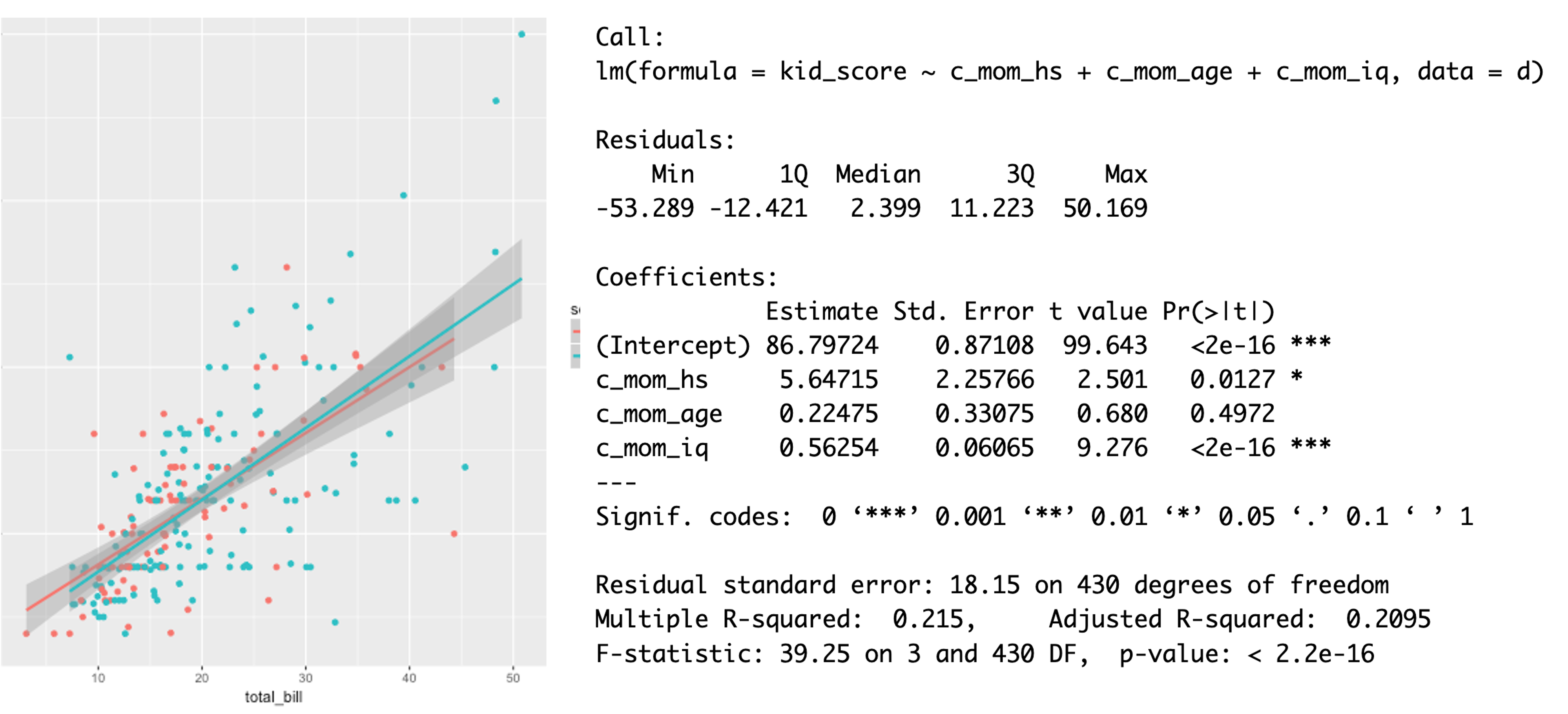
Model plots and model summaries are generated from our statistical analyses and look similar to the example below:

The image is an example of an effects plot (left) and model summary output (right). We, as communicators, need to tidy these up so that they are presentable. We do this and include them, with text, in the results sections of reports.
But what does the raw output contain? How do we use the information to understand what the data tells us?
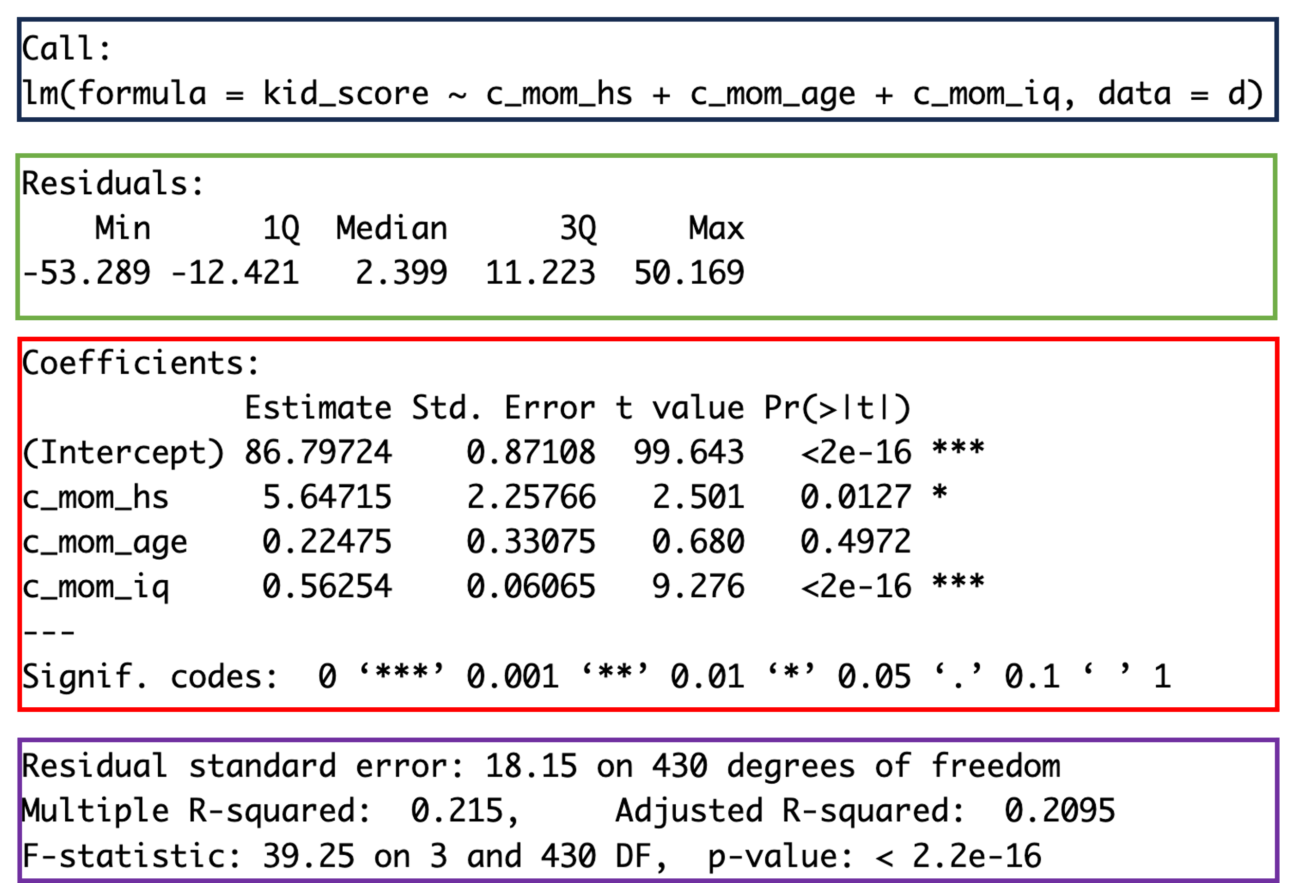
The raw model output is made up of four sections. From top to bottom, these are:

Call = the model formula. This is the line of code that represents the dependent and independent variables upon which the model is built
Residuals = the unexplained variance that is left over when the variance that is explained by the independent variables has been partialled out.
To do an eye-test of whether your model has not violated the assumption of normality, look at the Min, Max and the Median values in the Residuals section. Are the Min and Max values roughly the same numbers - but the Min has a minus sign? Is the Median value at zero or close to zero? If they are, then your model errors are probably normally distributed - which is good! And you can further verify with a test!
Coefficients = your results for each of the independent variables or predictors. Each row is for one predictor. Each column on each row is needed when you report a result for an individual predictor (see below for more detail).
Model Values (purple or bottom section) = these are statistics for the whole model. From this section, you want to report the F statistic, the p value and the Adjusted R2 (see below for more detail).
Remember: the two R2 values in the model summary are reported as proportions. They need to be multiplied by 100 and reported as a percentage in your results section.
Communicating Findings from Linear Regression Models
Any reporting of a linear regression model comes in two parts:
First we report the type of model, the model variables - outcomes & predictors (DVs and IVs in ANOVA langauge) and model statistics,
and then we report statistics for the individual coefficients from our hypotheses.
As an example, we can use the model summary from above.
Reporting the model
The information for the the first part of reporting the model is located at the top of the output, in the Call section, and the bottom of the output, in the Model Values section:
Example text for reporting model significance:
We conducted a multiple linear regression with children’s test scores as the outcome variable and mothers’ graduation status, age and intelligence scores as predictor variables. The model was significant (F (3, 430) = 39.25, p < .001) and explained 21% of the variance in children’s test scores.
Reporting an individual coefficient for an individual predictor
The information for the second part of reporting the model comes from the Coefficients section. Reporting the regression coefficient for an individual predictor that is statistically significant also happens in two parts:
Reporting the statistic (estimate and SE) and the significance (p value)
Reporting a verbal description of the effect
When a coefficient for a predictor was part of one of your hypotheses but is non-signficant in the model, then you only report part a. You do not report a verbal description of the effect.
The c_mom_hs is the coefficient label for the predictor that reflects a significant effect for whether a child’s mother completed high school or not. An example excerpt of text to report the finding for this predictor variable could be:
part a = Whether or not the mother graduated high school has a significant impact upon a child’s test score (b = 5.65, SE = 2.26, p = .013).
part b = Holding all other predictors constant, the difference in scores for a child whose mother finished high school and a child whose mother did not finish high school is 5.65 test points.
The c_mom_age is the coefficient label for the predictor that reflects a non-significant effect for the age of the mother at the time that the child takes the test. An example excerpt of text to report the finding for this predictor variable could be:
part a = The mother’s age at the time that the child took the test does not have a significant impact on a child’s test score (b = 0.22, SE = 0.33, p = .500).
There is no part b because the effect is non-significant.
Obviously, for the results section, these three excerpts are presented presented as a coherent body of text:
We conducted a multiple linear regression with children’s test scores as the outcome variable and mothers’ graduation status, age and intelligence scores as predictor variables. The model was significant (F (3, 430) = 39.25, p < .001) and explained 21% of the variance in children’s test scores.
Whether or not the mother graduated high school has a significant impact upon a child’s test score (b = 5.65, SE = 2.26, p = .013). Holding all other predictors constant, the difference in scores for a child whose mother finished high school and a child whose mother did not finish high school is 5.65 test points. The mother’s age at the time that the child took the test does not have a significant impact on a child’s test score (b = 0.22, SE = 0.33, p = .500).
Remember that values for means, SDs, coefficients and SEs, and p values all need to be reported to differing numbers of decimal places and rounded up! Go and find this in your personal source for your APA7 formatting guidance.
Use this model for reporting predictor effects across the next few weeks.
Staff role in labs
There will be two staff available during lab sessions. We will rotate around the room. You can raise your hand at any point to ask questions or get us to check your process as you go along.
In response, you can expect staff to:
- Tell you that there is an error somewhere with an indication of where to look more closely
- Give you hints
- Extend your thinking if you are working at your best level already….
We won’t give you the answers straight away. This is to encourage self-reliance and independence. Plus, there may be more than one correct answer to some of the questions.
Please don’t expect us to spend a lot of time with you if you have not watched the lecture beforehand.
Towards the end of each lab we will go through an example script of what could represent a way of working. There are mulitple example scripts that could all do the same job - so try not to think of the one that is presented as the “right” one or the only way to get to the output.