5. Factor Analysis and the Binomial Test

Emma Mills and Amy Atkinson

Introduction

This week is a crossover week between Emma and Amy.

Factor Analysis content is needed for learning. Questions will not be asked in the class test in week 20 on the Factor Analysis method.

The Binomial Test content is needed for learning, and the class test.

The rest of this page is split into two parts, Factor Analysis and Binomial Test. They each have their own associated lecture and notes.

Lecture

Watch the Lecture on Factor Analysis here

Slides

Please download the Slides. In this zipped folder are the slides that accompany the lecture and the codebook for the week 15 lab activity that uses the Birthweight dataset (which is associated with WBA5).

Week 15 Lab Activity

There are three scripts with associated data with which you can practise performing the steps of a factor analysis. These are in the folder called Three_Factor_Analyses.zip. It can be downloaded here. If you are completing the WBA Quizzes, then you will need to review the factor analysis for the Birthweight data to be able to complete WBA5.

Pre-Lab Activity

  1. Watch the lecture before you attempt anything!
  2. Download the Three_Factor_Analyses.zip files and upload to your R account
  3. Play with one of the scripts before the lab to familiarise yourself with the process - test yourself on WBA5
  4. Come to your scheduled lab to have a further practice and ask the staff questions about the process.

Test Yourself

The link to this week’s multiple choice quiz, WBA 5, is here

Factor Analysis

Factor analysis is an analysis method that aims to take a large number of observed variables, find subsets of the variables that are highly correlated with each other and construct a smaller set of unobserved variables, that we call latent variables.

Factor analysis assumes that when variables are very highly correlated with each other then on one level they could be measuring the same underlying construct. In which case, you can capture only the bits that contribute differentially to the underlying construct and make a new variable from those different parts.

A Diagram of a Factor Analysis Where 12 Observed Variables are Reduced to Four Latent Variables

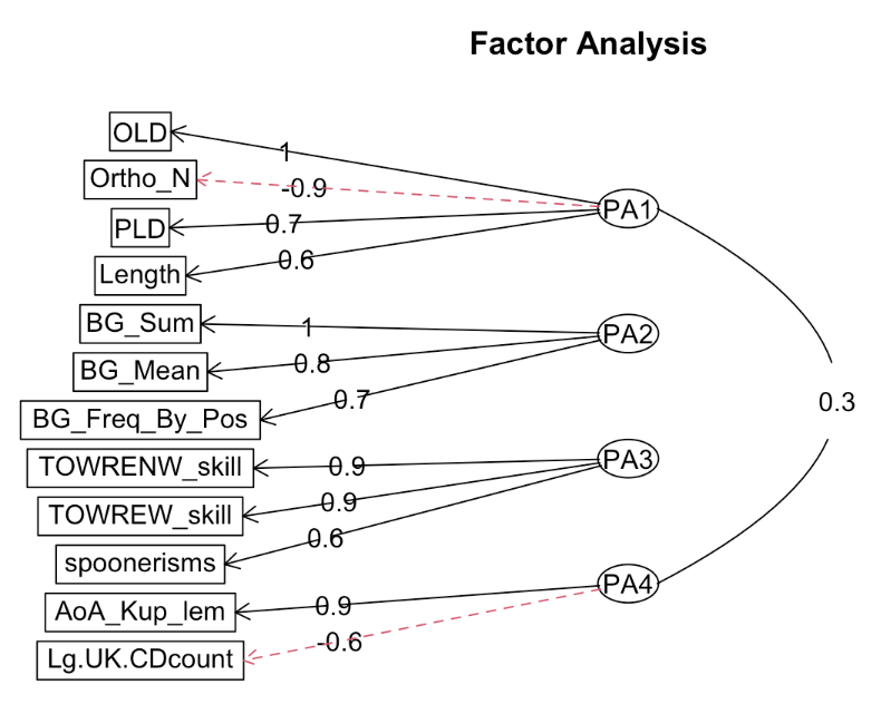
In this diagram, we have a set of observed variables on the left (rectangles). These are the constructs that we measure or observe. They are the columns that we can see in our dataset.

Moving across the page, most of the observed variables are connected by arrows to one of four latent variables (PA1, PA2, PA3, and PA4), on the right. Latent variables are always drawn in ovals or circles on these diagrams. These are the unobserved variables that are made during the factor analysis process.

What goes into the new, latent variables is decided by how well the observed variables correlate with each other. You have already been looking at how well predictor variables correlate with each other during the visualisation part of the analysis workflow (those complicated looking correlation matrices!). When subsets of observed variables correlate well with each other then this could be an indicator that a factor analysis is a feasible method for reducing a large set of variables down to a smaller set.

The values that you see on each of the connecting arrows are how much of the observed variable is contributing to the unobserved variables. We say this is an observed variable’s “loading” onto the latent variable. Higher loading values indicate stronger links to that latent variable.

In 224, you are engaging in questionnaire design, where sets of items are specifically designed to measure one construct. If you have three or more of those items, then you may have the conditions that suggest a factor analysis. In other studies, you may have taken a personality test, or other questionnaire style test where a lot of the questions seemed to ask about similar things. In the big five mini-IPIP scale, the two questions for extraversion are “Am the life of the party” and “Talk to a lot of different people at parties”. The expectation is that if there is indeed an underlying variable behind these two questions, then people’s responses should be similar to both questions.

Factor Analysis Needs Predictor Variables That Are Co-linear

Correlation looks at pairs of numerical variables

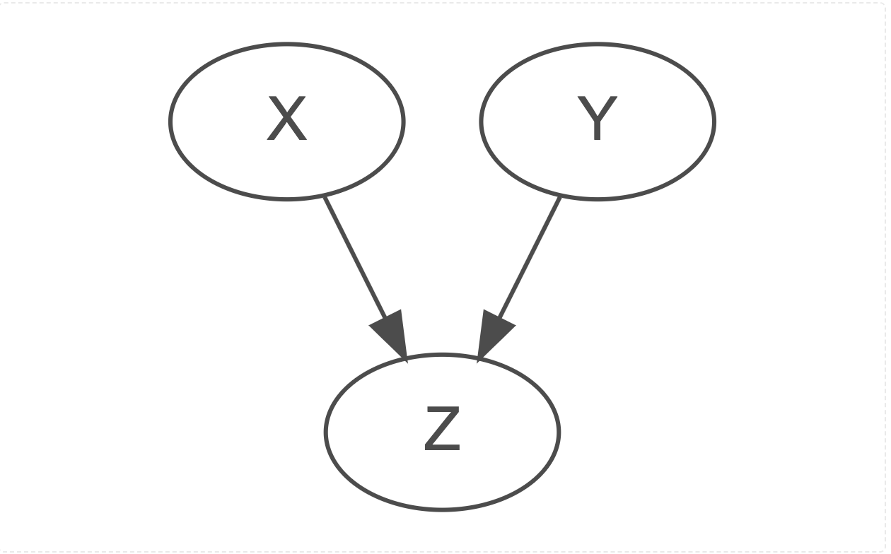
  • X and Y below predict Z
  • X and Y are completely separate
  • X and Y are completely independent of each other
  • X and Y are not correlated; they are not co-linear

Independent Predictors

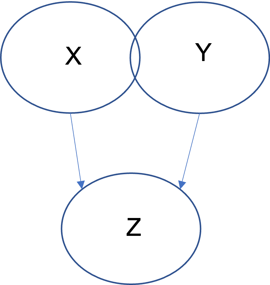
Here is an alternative way to show an independence between the two predictors:

Correlation of X and Y with Z, with X and Y Showing Complete Independence of Each Other
  • Again, X and Y both predict Z
  • X may be showing a stronger predictive relationship with Z, here (look at the overlap with Z compared to that between Y and Z)
  • And again, X and Y are completely separate
  • X and Y are completely independent of each other
  • They are not co-linear.

Sometimes the relationship between two predictors is not so independent:

Correlation of X and Y with Z, with X and Y Showing a Weak Correlation with Each Other

Here X and Y still predict Z, however now they are also correlated with each other, as described by the overlapping areas between X and Y. They share some information. They can be said to be co-linear (very weakly here), as well as being correlated or predicting Z.

We can draw the above diagram this way too…

An Alternative Way of Describing A Weakly Correlated Relationship Between Two Predictors

In this next diagram, the overlap between X and Y is now related to the overlap with Z to a much greater degree…however the correlation between the two predictors of X and Y remains weak.

Stronger Predictive Relationships for X and Y on Z, with a Remaining Weak Correlation Between X and Y

Multicollinearity

Weak correlations between predictor variables are not too problematic. If predictor variables share strong correlational relationships (normally r > .8), however, the algorithm that is doing the regression calculations for us (behind the scenes) will get a bit mixed up as it will not be able to to tell which predictor is predicting which bit of variance in the outcome variable. Predictors that share strong correlational relationships are fighting for the same part of the variance on Z.

Such strong correlational relationships between predictor variables are known as the predictor set having a high level of multicollinearity. Multicollinearity is likely to occur more in multiple regression simply because there are multiple predictor variables. This is one reason why it is a good idea to do a visualisation of the predictor variables in a correlation matrix, to see, at an early stage in an analysis, if multicollinearity is present. If it is, there are steps to mitigate its effect.

Mitigation

One way to mitigate multicollinearity is to simply leave some variables out of your dataset. There are estimation practices and methods that allow you to choose which to leave out in a principled, reproducible way.

Another way to mitigate multicollinearity is not to discard observed variables but to combine observed variables that are highly correlated together into one new latent variable. This is what a factor analysis method does. It calculates, across a set of otherwise correlated observed variables, what information is unique in a predictor for a hypothesised new variable and takes only sufficient information from each observed variables that uniquely contributes to the new variable. In this way, the multicollinearity amongst the observed variables is reduced with the relevant information from the observed variables retained and described by the new latent variables.

Theory should suggest which variables are likely to “load” together onto a latent variable. When this happens, you may engage in a “confirmatory factor analysis” or CFA. However, you can also take a data driven approach (by letting the model suggest loadings) if theory is agnostic, or variables are quite new. This is sometimes called an “exploratory factor analysis” or EFA.

Factor Analysis

Factor analysis is quite jargon heavy, it has its own little language system - annoying maybe, but you are familiar with the constructs that exist in regression already. They just have different labels in factor analysis.

  • Where there is overlap, where variables ‘load’ onto factors:
    • The shared variance is called ‘communality’.
    • And the unshared variance is called uniqueness.

Necessary Conditions

There are some conditions associated with making the new latent variables that must be met:

  • Latent variables should have three or more observed variables loading onto them.
  • Correlations between those three or more observed variables should be high (advice is given in the lab scripts).
  • Any one of the observed variables should load onto one latent variable only.
  • Before beginning your factor analysis, you should standardise your variables.
  • Ensure that reverse scored items are transformed to move in the same direction as the majority of the other variables

Performance

Example of 10 Predictor Loadings onto Four Latent Variables

Look at the table above. The first column is the labels of the observed variables. Columns 2 to 5 are the latent variable loadings for each of those observed variables.
- Look at the columns for PA1, PA2 and PA3. Each of those have more than three observed variables loading onto them.
- Look at the first row for the Length observed variable - see how it loads onto two of the latent variables, PA1 and PA2; this is problematic for this variable.

A good factor analysis should have:

  1. A factor should have at least three variables that are loaded to a sufficient level (see lab script for notes).
  2. Any one variable should have most of its loading on one factor
  3. A factor should have good internal consistency (a common (and maybe overused) method is Cronbach’s alpha).
  4. Factors should make theoretical sense.

Tidy your Dataset

  1. Remove outcome variables, categorical variables and ordinal variables

  2. Visualise the prepared dataset.

  3. Inspect correlations between the remaining predictors (guidelines exist!)

  4. Perform some specific tests to determine if a factor analysis is feasible (all in the lab script)

    • KMO
    • Bartlett’s test of sphericity
    • Parallel analysis
    • Scree test (visualization)
  5. If the indications are good and you have a sufficient number of variables– then perform a factor analysis

Model / Perform your Factor Analysis

Running the factor analysis takes but a moment. It is the checking and interpretation that takes the time for this process. In the lab script, there are guidelines for the following steps of deciding whether a factor analysis is a good fit for the data:

  1. Look for patterns inside the new, suggested latent factors

  2. Look for patterns between the new, suggested latent factors

  3. Look for communalities

  4. Look for factor correlations

  5. Test for internal consistency of the factors

  6. Draw!

  7. Report!

Binomial Test

Lecture material

Watch part two of the Week 15 lecture (on the binomial test) here. The lecture slides (both .ppt and .pdf) versions can be downloaded here.

Running the code in the lecture

Please note that binomial test will not be covered in the Week 15 lab - as described in the lecture, this is a very straightforward test to run in R that can be performed with just a single line of code.

To run the binomial test based on the example described in the lecture, you would simply run the following code in R:

binom.test(13, 14, 0.5)

    Exact binomial test

data:  13 and 14
number of successes = 13, number of trials = 14, p-value = 0.001831
alternative hypothesis: true probability of success is not equal to 0.5
95 percent confidence interval:
 0.6613155 0.9981932
sample estimates:
probability of success 
             0.9285714 

Independent learning activities

Below are some independent learning activities you can have a go at to help consolidate the lecture content on the binomial test. These are optional, but recommended. The answers are found below.

Activity 1

One sample-test or binomial test?

Disclaimer: All of these statistics are made up.

For the following examples, write down whether you think the test conducted should be a one-sample t-test or a binomial test.

  1. You are the coach of a football team. You are interested in whether the running distance of your players significantly differs from the England national football team. You know, on average, England football players run 10km per game.

  2. You are the coach of a football team. You are interested in whether the proportion of games your team scores a goal is significantly different from that of the England national team. You know that on average, the England national team scores a goal in 60% of games.

  3. You are a neonatal doctor (a doctor who specialising in caring for newborn babies). You think that babies born in your hospital are quite small. You are interested in whether the proportion of babies who are classed as “small for gestational age” differs between your hospital and the UK average (10%).

  4. You are a neonatal doctor (a doctor who specialising in caring for newborn babies). You think that babies that are born in your hospital are quite small. You are interested in whether the average weight of babies born at your hospital is significantly less than the UK average (3350g).

Activity 2

Identifying “success”

  1. You are the headteacher of a grammar school which has an entrance exam. You are interested in whether the proportion of children failing the test differs significantly from last year. The failure rate last year was 24% (or 0.24 expressed as a proportion).

  2. You have developed a new flu vaccine. You are interested in whether the proportion of people who develop side effects after your vaccine differs from the flu vaccine currently used by the NHS (37%, or 0.37 expressed as a proportion).

Answers

Activity 1:

  1. One-sample t-test. The value for each individual is continuous.You are interested in whether the mean number of km runs differs from a known value.

  2. Binomial test. Two possible outcomes: team scores or team does not score). You are interested in whether the proportion that a given outcome occurs (i.e. your team scores a goal) differs from a known value.

  3. Binomial test. Two possible outcomes: Each baby’s outcome is either “small for gestational age” or “not small for gestational age”. You are interested in whether the proportion that a given outcome occurs (i.e. small for gestational age) differs from a known value.

  4. One-sample t-test. The value for each individual is continuous. You are interested in whether the mean weight of babies at your hospital differs from a known value.

Take-home message: A one sample t-test is used when you are interested in comparing the mean of a sample to a known value. The binomial test is used when you are interested in comparing a sample’s proportion of “successes” to a known value.

Activity 2

  1. Success: failing the test. Failure: passing the test.

  2. Success: Has side effects. Failure: Does not have side effects.

Take home message: Success refers to the outcome you are interested in. Sometimes this might be counterintuitive to how we typically think about ‘success’ (e.g. in the.

Asking questions

If you have any questions about the binomial test, please post them on the discussion board here. If you prefer to remain anonymous, you can post questions anonymously here: “The Binomial Test: Post questions anonymously”. I will then copy your question to the discussion forum and answer it there and/or cover it in next Q&A session.

Back to top