This week, there are three mini lectures, and the practical workbook working with R-studio.
Before the practical on Tuesday, please try to work through the practical workbook in your group.
Bring your questions (and/or answers) to the practical.
4.2 Learning Goals
Understand the value of conducting statistical tests and interpreting p-values
Understand null effects and null hypotheses
Understand the difference between parametric and non-parametric data
Understand when to apply the Chi-squared test
Understand the relation between Cramer’s V test and the Chi-squared test
Be able to apply the Chi-squared test to data and interpret the result
Be able to apply Cramer’s V test to data
4.3 Lectures and slides
4.3.1 Lectures
Watch Lecture week 4 part 1:
Watch Lecture week 4 part 2:
Watch Lecture week 4 part 3:
Note on typo in week 4 part 3
Please note for the part 3 recording, the screen shows PSYC401 instead of PSYC411 in places. I am reluctant to go in and correct this typo as panopto recordings aren’t working very well for me at the moment. So, please excuse the error! It should be PSYC411.
Take the quiz (not assessed) on the lecture materials.
In your group, work through this workbook, note any problems and questions you have, and come prepared to the online practical class to go through the tasks and ask your questions.
4.4.1.1 Part 1: Revision for last week
Task 1: Your graphs on the vocabulary scores data
One of the tasks from last week was to produce some graphs of the data set PSYC411-shipley-scores-anonymous-17_18.csv. Go back to your Week 3 rscript to remind yourself of the relations you looked at in your graphs, and discuss what they might mean in your group.
OK, revision is over.
4.4.1.2 Part 2: Load in the New Vocabulary Scores Data and Produce Graphs
Task 2: Load in the Data
We will now look at the vocabulary scores data updated to include your own data. Make a new script for this week, called psyc411_week3.r or another name that makes sense to you.
Remember to clear out R first and load the tidyverse library:
rm(list=ls())library(tidyverse)
Warning: package 'ggplot2' was built under R version 4.4.3
── Attaching core tidyverse packages ──────────────────────── tidyverse 2.0.0 ──
✔ dplyr     1.1.4     ✔ readr     2.1.5
✔ forcats   1.0.0     ✔ stringr   1.5.1
✔ ggplot2   4.0.1     ✔ tibble    3.2.1
✔ lubridate 1.9.4     ✔ tidyr     1.3.1
✔ purrr     1.0.4
── Conflicts ────────────────────────────────────────── tidyverse_conflicts() ──
✖ dplyr::filter() masks stats::filter()
✖ dplyr::lag()    masks stats::lag()
ℹ Use the conflicted package (<http://conflicted.r-lib.org/>) to force all conflicts to become errors
The data set on the Shipley and Gent vocabulary scores is now updated with the data from your group, so it now contains nine years of PSYC411 students’ data. There are three datasets, I have separated the data in order to preserve anonymity, and changed the subject_ID numbers.
The first contains information about vocabulary scores and gender - this is called PSYC411-shipley-scores-anonymous-17_25_gender.csv. Download this file to your computer, then Upload it into the r server. Save it as an object in R studio called vocabgenderdat.
The second contains information about vocabulary scores and language background and year of academic study - this is called PSYC411-shipley-scores-anonymous-17_25_year_language.csv and read the data into an object in R studio called vocabyearlangdat (for vocabulary data).
The third contains information about gender and language background - this is called PSYC411-shipley-scores-anonymous-17_25_gender_language.csv and read the data into an object in R studio called genderlangdat (for vocabulary data).
Rows: 293 Columns: 5
── Column specification ────────────────────────────────────────────────────────
Delimiter: ","
chr (1): Gender
dbl (4): subject_ID, Shipley_Voc_Score, Gent_1_score, Gent_2_score

ℹ Use `spec()` to retrieve the full column specification for this data.
ℹ Specify the column types or set `show_col_types = FALSE` to quiet this message.
Rows: 293 Columns: 7
── Column specification ────────────────────────────────────────────────────────
Delimiter: ","
chr (1): english_status
dbl (6): subject_ID, Age, Shipley_Voc_Score, Gent_1_score, Gent_2_score, aca...

ℹ Use `spec()` to retrieve the full column specification for this data.
ℹ Specify the column types or set `show_col_types = FALSE` to quiet this message.
Rows: 293 Columns: 3
── Column specification ────────────────────────────────────────────────────────
Delimiter: ","
chr (2): english_status, Gender
dbl (1): subject_ID

ℹ Use `spec()` to retrieve the full column specification for this data.
ℹ Specify the column types or set `show_col_types = FALSE` to quiet this message.
As a reminder, when we want to look at a particular variable (a column) in an object in R studio, we refer to it using the $ notation. So, for the object vocabyearlangdat and the variable academic_year you would refer to it as vocabyearlangdat$academic_year. For this data set, we need to change academic year to be a nominal (factor) variable. Why are we setting academic year to be nominal and not interval/ratio?:
vocabyearlangdat$academic_year <-as.factor(vocabyearlangdat$academic_year)# View(vocabyearlangdat) #view the data
Answer
It has to be nominal unless we have a hypothesis about the order of years of groups being important to the data. But that is very unlikely to have an effect (though you could look up the “Flynn Effect” in case you wanted to generate one…). But for now we want each year to be treated independently, rather than in order, in our analysis.
Make sure the tidyverse library is loaded. Select all the variables apart from Age and save as a new object called “summaryvdat”. We will omit these variables because they are not complete for the dataset.
Hint
# there are two ways to do this, either list the variables you are omitting with a `-c(variables,variables,...)` command:summaryvdat <-select(vocabyearlangdat, -c(Age))# or list the variables we do want to include:summaryvdat <-select(vocabyearlangdat, subject_ID, english_status, Shipley_Voc_Score, Gent_1_score, Gent_2_score, academic_year)
Arrange the data according to Gent_2_score, from highest to lowest. Save this as a new object called “summaryvdat_sort”
Draw graphs of the following relations using the summaryvdat object:
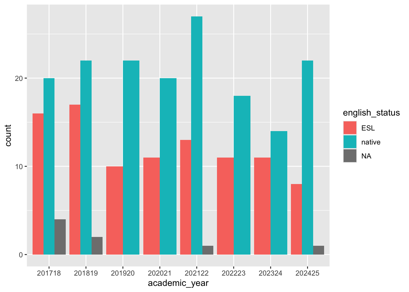
English status and academic year
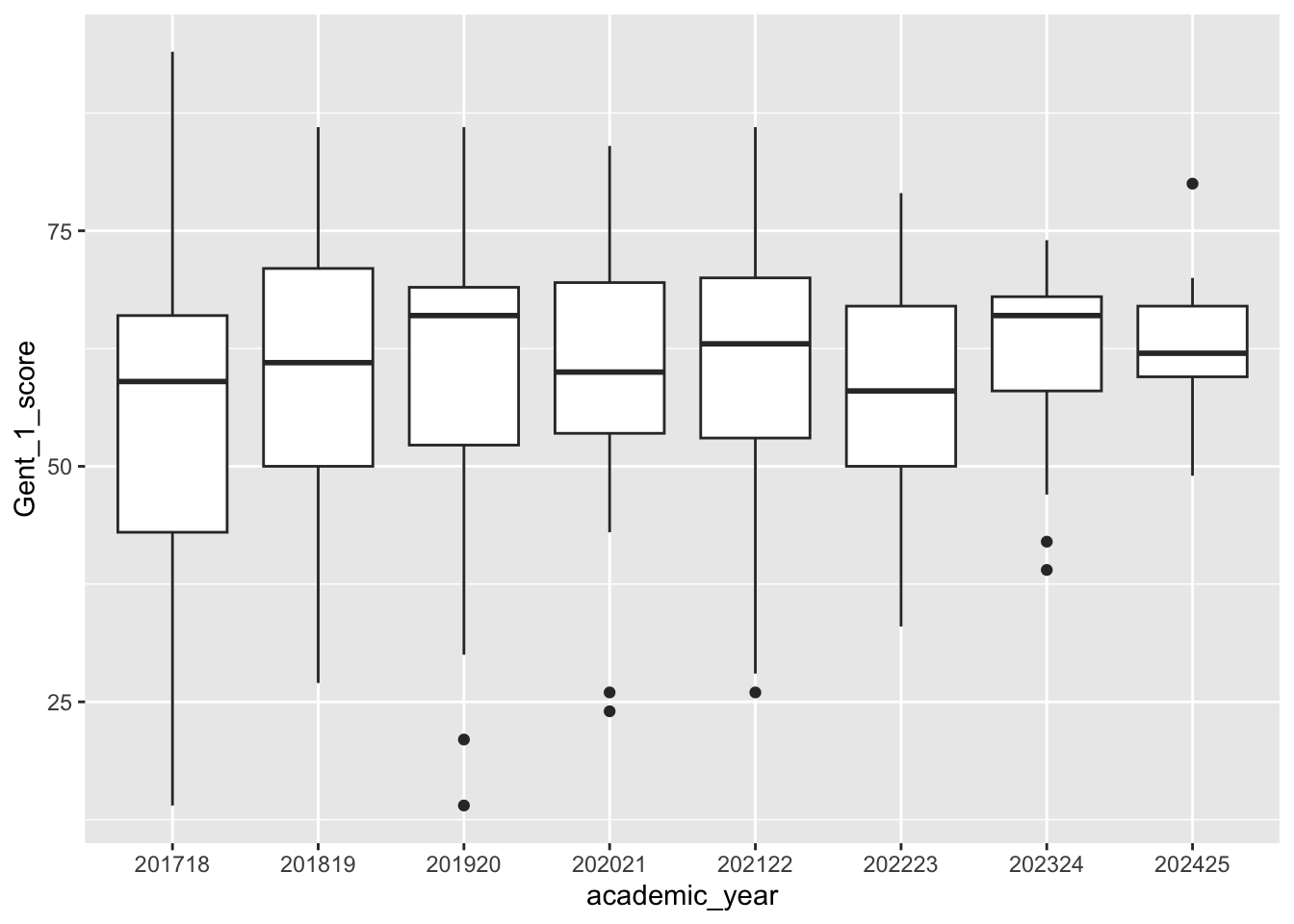
Vocabulary score and academic year (choose any of the vocabulary measures) Using the vocabgenderdat object, draw a graph of the relations between:
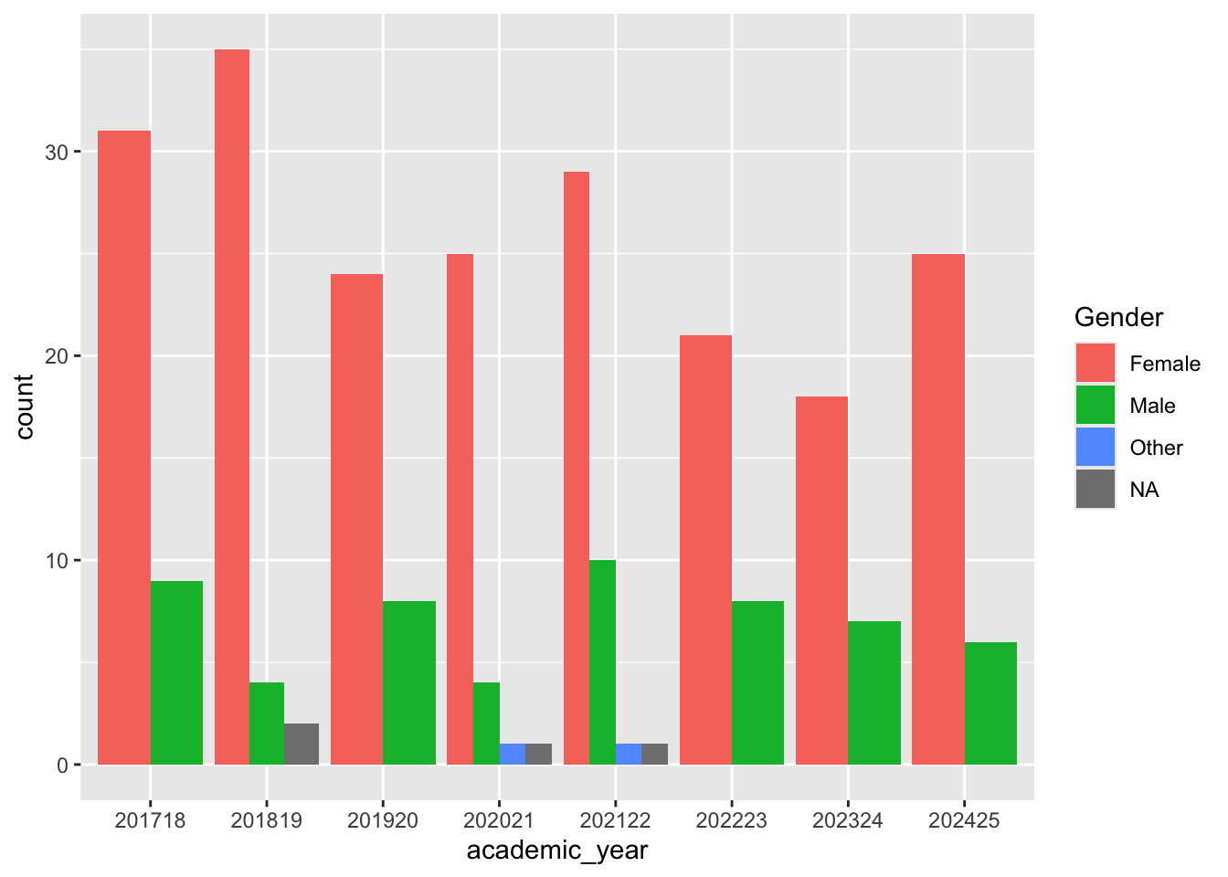
Vocabulary score and gender And using the genderlangdat object, draw a graph of the relations between:
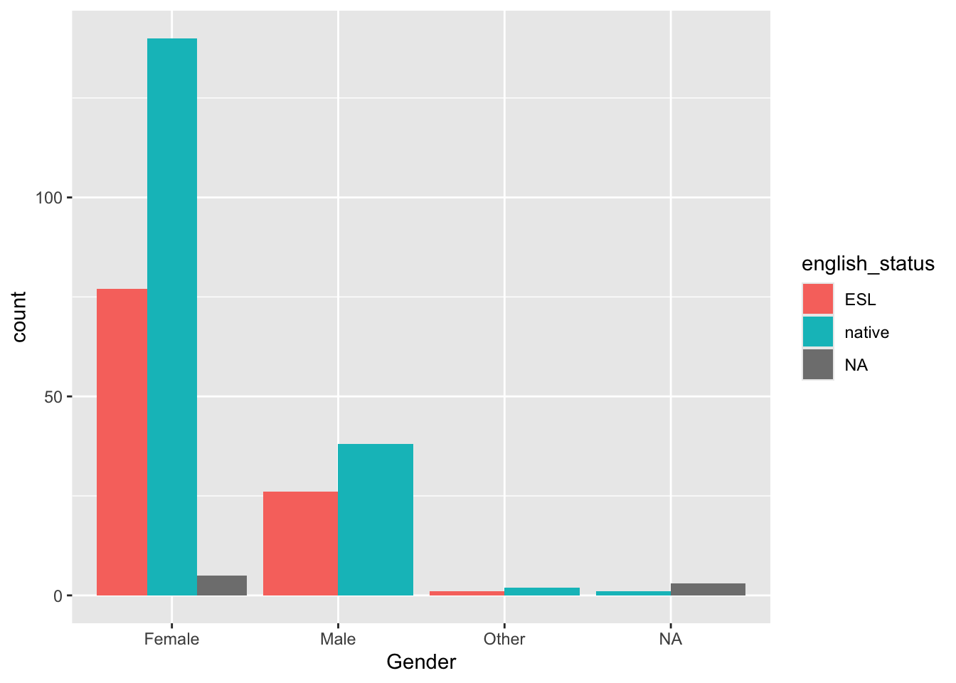
gender and english status (language)
Answer
ggplot(summaryvdat, aes(x = academic_year, fill = english_status)) +geom_bar(position ="dodge")
ggplot(summaryvdat, aes(x = academic_year, y = Gent_1_score)) +geom_boxplot()
Warning: Removed 5 rows containing non-finite outside the scale range
(`stat_boxplot()`).
ggplot(vocabgenderdat, aes(x = Gender, y = Gent_1_score)) +geom_boxplot()
Warning: Removed 5 rows containing non-finite outside the scale range
(`stat_boxplot()`).
ggplot(genderlangdat, aes(x = Gender, fill = english_status)) +geom_bar(position ="dodge")
Save your script file.
4.4.1.3 Part 3: Grouping data in R studio
Task 4: Loading and joining data in R studio
Now, let’s clear out R-studio before we get started again using rm(list=ls()).
Go to the data files from week 2 and load them into Rstudio again (“ahicesd.csv”, and “participantinfo.csv”). If you need to download these again, you can get them here: ahicesd.csv, participantinfo.csv.
Remember these data come from this study: Woodworth, R.J., O’Brien-Malone, A., Diamond, M.R. and Schuz, B. (2018). Data from, “Web-based Positive Psychology Interventions: A Reexamination of Effectiveness”. Journal of Open Psychology Data, 6(1).
Remind yourself of the aim of the study and the variables that are in the data set (see end of this script file for repeat description on the study).
Next, load and join the ahicesd.csv and participantinfo.csv data in R studio. Call the joined data set “all_dat” (see week 2 workbook for reminders about this)
Rows: 992 Columns: 50
── Column specification ────────────────────────────────────────────────────────
Delimiter: ","
dbl (50): id, occasion, elapsed.days, intervention, ahi01, ahi02, ahi03, ahi...

ℹ Use `spec()` to retrieve the full column specification for this data.
ℹ Specify the column types or set `show_col_types = FALSE` to quiet this message.
pinfo <-read_csv("data/wk2/participantinfo.csv")
Rows: 295 Columns: 6
── Column specification ────────────────────────────────────────────────────────
Delimiter: ","
dbl (6): id, intervention, sex, age, educ, income

ℹ Use `spec()` to retrieve the full column specification for this data.
ℹ Specify the column types or set `show_col_types = FALSE` to quiet this message.
all_dat <-inner_join(x = dat, y = pinfo, by =c("id", "intervention"))
Task 5: Selecting and manipulating data
We’re not interested in the individual questionnaire items. So, let’s select all the variables we want to keep (omitting the individual questionnaire items), and save this to an object called summary_all_dat (again see week 2 workbook for reminder)
Next, we will add another variable to the data. We use the function mutate() for this. Let’s scale the ahiTotal and cesdTotal values and add them to the summary_all_dat set.
What are the minimum and maximum values of the new variable ahiTotalscale?
What do these scale values mean? (reminder: they are Z scores).
Hint
hint: use the arrange() function, or the min() and max() functions.
The values are z-scores so the numbers indicate how many standard deviations the values are from the mean
The next way we will work with the data is to organise the observations into different groups. We will use the function summarise(). So, instead of mean(summary_all_dat_scale$ahiTotal) you can use this, which turns out to be a much more powerful way of looking at the data:
summarise(summary_all_dat_scale, mean(ahiTotal))
They should give the same results - check that they do. This function summarise() is more powerful because you can look at several values at the same time, e.g.:
But now let’s think about what kind of patterns we’d like to investigate in the data. There are four interventions conducted in this study. Let’s look at each of these interventions and their effect of ahiTotal and cesdTotal.
We can look at subgroups of data either by using the filter() function, or by using the function group_by(). The advantage of group_by() is that we can look at several groups at the same time, rather than dividing up the data file into pieces. Let’s organise by the different interventions.
This command takes the data summary_all_dat_scale, and then groups it according to the four interventions in the data. We can’t yet see any difference in summary_all_dat_scale_intervention but it’s in there, lurking, just waiting.
Now, we can look at the means for each intervention using the summarise function again. Run the summarise function on summarydata_scale_intervention. What happens?
It separates out the means and SDs by the group_by condition - i.e, by intervention.
You can also group by several factors at the same time. We can group by intervention and get means and standard deviations, but that is not going to give us a huge amount of insight into how the interventions affect the happiness measure because we are combining the mean of ahiTotal across all occasions of testing, including testing before the intervention has been applied.
So, let’s group by intervention and occasion of testing:
This doesn’t print all the lines out, so you can make a new object (e.g., called sum_output) and view that, or you can filter out some of the lines so we only look at the first and second occasion of testing.
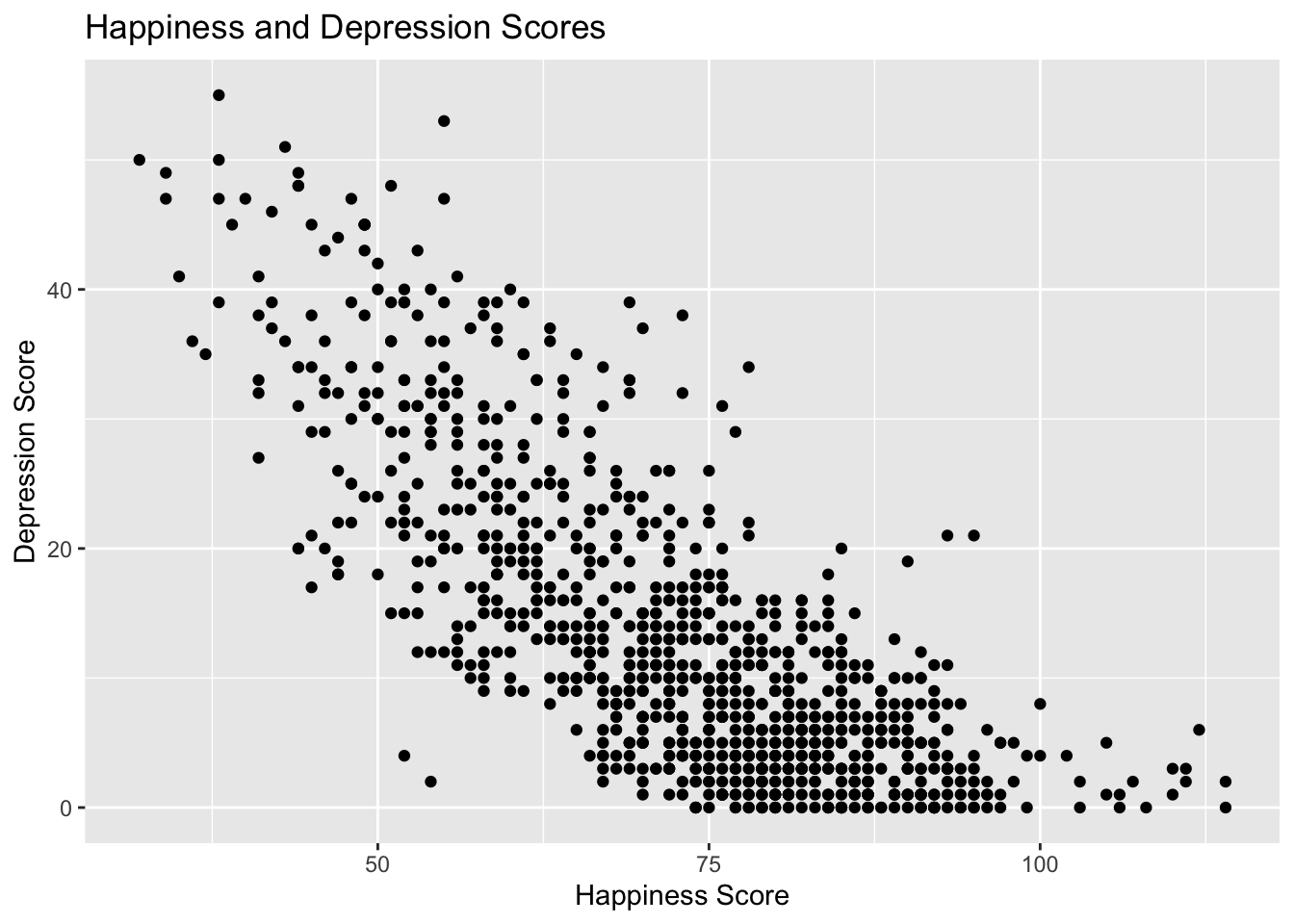
Draw a scatter plot of ahiTotal and cesdTotal values for the whole data set.
Hint
Use the ggplot() function with geom_point()
And make it a bit more beautiful using the labs() addition.
Answer
ggplot(summary_all_dat, aes(x = ahiTotal, y = cesdTotal)) +geom_point() +labs(title ="Happiness and Depression Scores", x ="Happiness Score", y ="Depression Score")
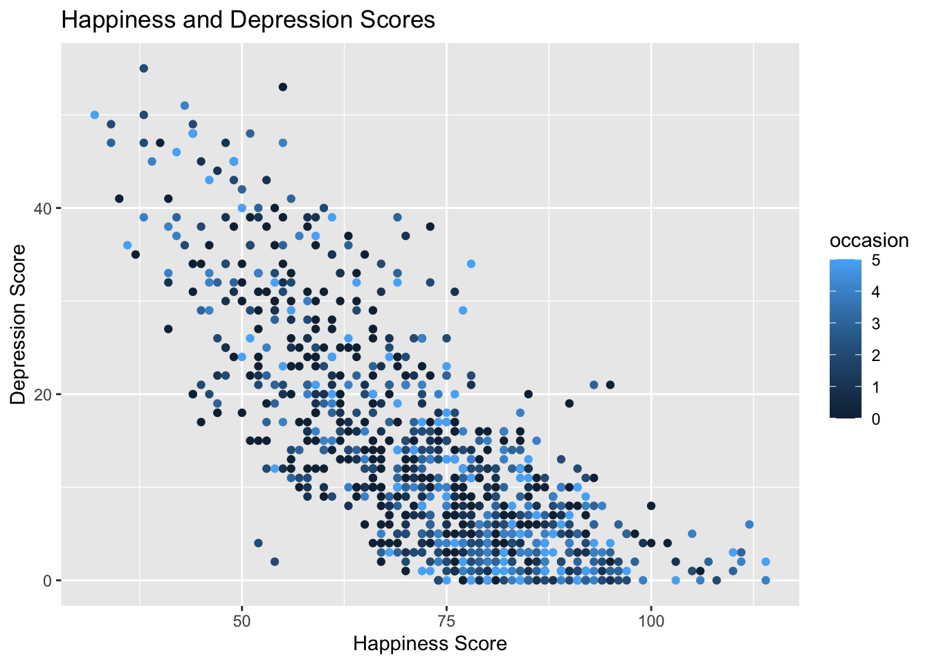
Now redraw the plot, but colour the points according to whether they are first, second, third, etc occasion of testing. Add in col = "occasion" into the aes() part of the geom_point function, so that this part looks like this: aes(x = ahiTotal, y = cesdTotal, col = occasion)
Answer
ggplot(summary_all_dat, aes(x = ahiTotal, y = cesdTotal, col = occasion)) +geom_point() +labs(title ="Happiness and Depression Scores", x ="Happiness Score", y ="Depression Score")
4.4.1.5 Part 5: Working out whether nominal data is random or structured: Repeating the analyses from Lecture week4 part3
Task 7: Chi-squared and Cramer’s V
Let’s now have a look at running Chi-squared and Cramer’s V tests in R. Download the titanic data.
Read the titanic.csv into an object called “titanic”.
View the data. It should correspond to the data in the overhead slides.
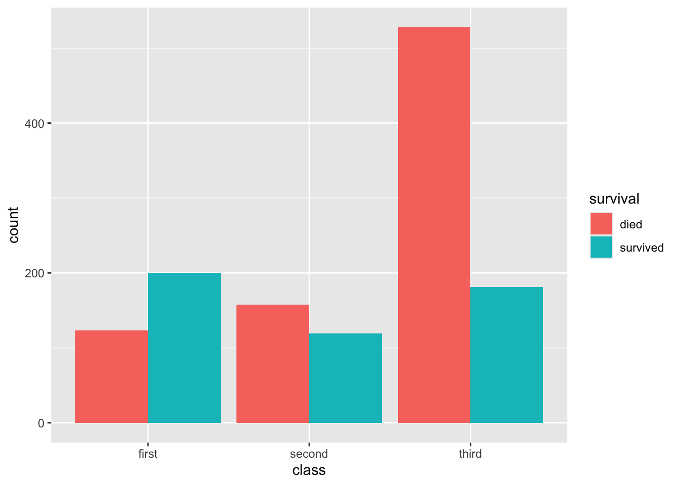
Make a bar graph to count the numbers of survived and died by class.
Answer
titanic <-read_csv("data/wk4/titanic.csv")
New names:
Rows: 1309 Columns: 3
── Column specification
──────────────────────────────────────────────────────── Delimiter: "," chr
(2): class, survival dbl (1): ...1
ℹ Use `spec()` to retrieve the full column specification for this data. ℹ
Specify the column types or set `show_col_types = FALSE` to quiet this message.
• `` -> `...1`
ggplot(titanic, aes(x = class, fill = survival)) +geom_bar( position ="dodge")
Now let’s see if there is a significant relation between class and survival using Chi-squared:
chisq.test(x = titanic$class, y = titanic$survival)
The results give the chi-squared value, the number of degrees of freedom, and the p-value. P = 2.2e-16 means p = .0000000000000022. That’s highly significant. That means the observations are divided across the categories in a way that is very unlikely to be due to chance (for this number (P = 2.2e-16), it means there’s a 2 in a quadrillion chance that titanic survival was not related to class).
In a report, you would write:
X-squared(2, N = 1309) = 127.86, p < .001.
To understand where the significant effect comes from, we need to look at where in our table of counts there is a big discrepancy between the expected frequency and the actual frequency. We can do this by analysing the “standardised residuals” of the chi-squared test.
Repeat the chi-squared test on the titanic data set, and save the result of the test into a new object called “titanic_chisq_result”.
Then, look at the standardised residuals that are saved in the test results - the standardised residuals are saved in a variable called stdres.
Hint
Here is how you do it
titanic_chisq_result <-chisq.test(x = titanic$class, y = titanic$survival)titanic_chisq_result$stdres
             titanic$survival
titanic$class       died   survived
       first  -10.110480  10.110480
       second  -1.837589   1.837589
       third   10.254442 -10.254442
Negative values indicate that actual counts are lower than expected, positive values indicate that actual counts are higher than expected. The standardised residuals indicate that there are fewer first class and more third class than expected that died, second class died at a level close to that expected from the overall numbers of deaths.
Now, let’s compute Cramer’s V. First, we need to make sure we have the library lsr loaded in.
library(lsr)
Then run the test:
cramersV(x = titanic$class, y = titanic$survival)
Your next task is to run some Chi-squared and Cramer’s V tests on some of the other nominal data. Open the data “PSYC411-shipley-scores-anonymous-17_25_gender_language.csv” again. Investigate the association between gender and english status (are there different distributions of males and females for those with English as a first or additional language) using Chi-squared and Cramer’s V. Is it significant?
Rows: 293 Columns: 3
── Column specification ────────────────────────────────────────────────────────
Delimiter: ","
chr (2): english_status, Gender
dbl (1): subject_ID

ℹ Use `spec()` to retrieve the full column specification for this data.
ℹ Specify the column types or set `show_col_types = FALSE` to quiet this message.
chisq.test( x = genderlangdat$Gender, genderlangdat$english_status)
Warning in chisq.test(x = genderlangdat$Gender, genderlangdat$english_status):
Chi-squared approximation may be incorrect
    Pearson's Chi-squared test

data:  genderlangdat$Gender and genderlangdat$english_status
X-squared = 0.57694, df = 2, p-value = 0.7494
cramersV( x = genderlangdat$Gender, genderlangdat$english_status)
Warning in stats::chisq.test(...): Chi-squared approximation may be incorrect
[1] 0.0450721
It is not significant, X-squared(2, N = 284) = 0.58, p = .749, Cramer’s V = 0.05, but note that there is < 5 in the “Other” gender category which gives us the warning message “Chi-squared approximation may be incorrect”.
If we focus just on Male/Female data, if, for instance, we are interested for the purposes of our investigation only in these larger categories:
genderlangdatmf <-filter(genderlangdat, Gender =="Male"| Gender =="Female")chisq.test( x = genderlangdatmf$Gender, genderlangdatmf$english_status)
    Pearson's Chi-squared test with Yates' continuity correction

data:  genderlangdatmf$Gender and genderlangdatmf$english_status
X-squared = 0.36297, df = 1, p-value = 0.5469
cramersV( x = genderlangdatmf$Gender, genderlangdatmf$english_status)
[1] 0.03594057
It still is not significant, X-squared(1, 281) = 0.36, p = .547, Cramer’s V = 0.04.
What about the association between english_status and year?
Rows: 293 Columns: 7
── Column specification ────────────────────────────────────────────────────────
Delimiter: ","
chr (1): english_status
dbl (6): subject_ID, Age, Shipley_Voc_Score, Gent_1_score, Gent_2_score, aca...

ℹ Use `spec()` to retrieve the full column specification for this data.
ℹ Specify the column types or set `show_col_types = FALSE` to quiet this message.
chisq.test( x = vocabyearlangdat$academic_year, vocabyearlangdat$english_status)
    Pearson's Chi-squared test

data:  vocabyearlangdat$academic_year and vocabyearlangdat$english_status
X-squared = 4.746, df = 8, p-value = 0.7843
cramersV( x = vocabyearlangdat$academic_year, vocabyearlangdat$english_status)
[1] 0.1290454
It is not significant, X-squared(8, 285) = 4.75, p = .784, Cramer’s V = 0.13.
4.4.1.6 Part 6: More practice using Chi-squared and Cramer’s V test
Task 8: More Chi-squared and Cramer’s V tests
Look at the “ahicesd.csv” and “participantinfo.csv” data sets from week 2 again. Which nominal measures could you look at an association between? Report the Chi-squared test and Cramer’s V results for these associations. Are these associations significant? How do you interpret the significant associations?
Answer
For example, you could have a go at occasion and intervention. This would tell you whether the participants are unevenly distributed across the occasions and interventions:
a <-group_by(all_dat, occasion, intervention)chisq.test( x = all_dat$occasion, all_dat$intervention)
    Pearson's Chi-squared test

data:  all_dat$occasion and all_dat$intervention
X-squared = 9.7806, df = 15, p-value = 0.8333
cramersV( x = all_dat$occasion, all_dat$intervention)
[1] 0.05732779
It is not significant: X-squared(15, N = 992) = 9.78, p = .833, Cramer’s V = 0.06. We do not have evidence that there are different distributions of participants across the occasions and interventions.
4.4.1.7 Part 7: Extra practise downloading and analysing data
Here is another dataset for you to investigate:
Papoutsi, C., Zimianiti, E., Bosker, H. R., & Frost, R. L. (2024). Statistical learning at a virtual cocktail party. Psychonomic Bulletin & Review, 31(2), 849-861. https://doi.org/10.3758/s13423-023-02384-1
The data are available on OSF, but also a cleaned version of the dataset is available here. If this doesn’t work when you try to upload into psy-rstudio.lancaster.ac.uk, then you can always get the data from the osf site using this command:
dat <-read_csv('https://osf.io/download/ky4u6/')
There is also something in the osf site called a R-markdown file - Data_analysis_script.rmd
This is a special kind of R-script, a “R-markdown” file, which also stores the results alongside the commands.
You should be able to scroll through it and see some of the R studio commands that might be familiar.
Our challenge to you is to make a Figure that looks a bit like their Figure 2. e.g., construct a boxplot of some of these data (though the Figure they use is called a pirate plot). If you’re keen to learn, there is more information on pirate plots here: pirateplots
Rows: 10236 Columns: 24
── Column specification ────────────────────────────────────────────────────────
Delimiter: ","
chr (13): participant, test, test_speaker, word1, word2, test_type, testpair...
dbl (11): trialNo, tablerow, soundrow, correct_answer, rt, status, trialaccu...

ℹ Use `spec()` to retrieve the full column specification for this data.
ℹ Specify the column types or set `show_col_types = FALSE` to quiet this message.
Have a further browse of Psychological Science for data sets that you can download and begin to explore. Practise applying the data manipulation and graphing functions to these data sets. Or here is another one you might find interesting:
Woodworth, R. J., O’Brien‐Malone, A., Diamond, M. R., & Schüz, B. (2017). Web‐based positive psychology interventions: A reexamination of effectiveness. Journal of Clinical Psychology, 73(3), 218-232. Data available here
Description of their study:
In our study we attempted a partial replication of the study of Seligman, Steen, Park, and Peterson (2005) which had suggested that the web-based delivery of positive psychology exercises could, as the consequence of containing specific, powerful therapeutic ingredients, effect greater increases in happiness and greater reductions in depression than could a placebo control. Participants (n=295) were randomly allocated to one of four intervention groups referred to, in accordance with the terminology in Seligman et al. (2005) as 1: Using Signature Strengths; 2: Three Good Things; 3: Gratitude Visit; 4: Early Memories (placebo control). At the commencement of the study, participants provided basic demographic information (age, sex, education, income) in addition to completing a pretest on the Authentic Happiness Inventory (AHI) and the Center for Epidemiologic Studies-Depression (CES-D) scale. Participants were asked to complete intervention-related activities during the week following the pretest. Futher measurements were then made on the AHI and CESD immediately after the intervention period (‘posttest’) and then 1 month after the posttest (day 38), 3 months after the posttest (day 98), and 6 months after the posttest (day 189). Participants were not able to to complete a follow-up questionnaire prior to the time that it was due but might have completed at either at the time that it was due, or later. We recorded the date and time at which follow-up questionnaires were completed.